
機械学習:R言語(Tidymodels)チュートリアルの和訳①

R言語を普及したい!
機械学習楽しいよ!
Kaggleにも挑戦できるよ!!
という事で、自分の復習もかねてチュートリアルを和訳します。
※細かい文章は省略しています。
対象のチュートリアル
ホテルの宿泊データ
まず、ライブラリを使えるようにします。
library(tidymodels)
library(readr)       # for importing data
library(vip)         # for variable importance plots
予測タスクの目的:ゲストが子供や赤ちゃんを含むホテルの滞在を予測する
library(readr) hotels <- read_csv("https://tidymodels.org/start/case-study/hotels.csv") %>%
mutate(across(where(is.character), as.factor))
※キャンセルした人のデータには欠損が多いため、キャンセルしていない人のみのデータで分析を行う
glimpse(hotels) は、データセットをざっくりと表示するコマンドです。
hotelから始まる縦列がデータの変数(列)です。
予測するものは「children」です(2値)。
glimpse(hotels)
#> Rows: 50,000
#> Columns: 23
#> $ hotel                          <fct> City_Hotel, City_Hotel, Resort_Hotel, R…
#> $ lead_time                      <dbl> 217, 2, 95, 143, 136, 67, 47, 56, 80, 6…
#> $ stays_in_weekend_nights        <dbl> 1, 0, 2, 2, 1, 2, 0, 0, 0, 2, 1, 0, 1, …
#> $ stays_in_week_nights           <dbl> 3, 1, 5, 6, 4, 2, 2, 3, 4, 2, 2, 1, 2, …
#> $ adults                         <dbl> 2, 2, 2, 2, 2, 2, 2, 0, 2, 2, 2, 1, 2, …
#> $ children                       <fct> none, none, none, none, none, none, chi…
#> $ meal                           <fct> BB, BB, BB, HB, HB, SC, BB, BB, BB, BB,…
#> $ country                        <fct> DEU, PRT, GBR, ROU, PRT, GBR, ESP, ESP,…
#> $ market_segment                 <fct> Offline_TA/TO, Direct, Online_TA, Onlin…
#> $ distribution_channel           <fct> TA/TO, Direct, TA/TO, TA/TO, Direct, TA…
#> $ is_repeated_guest              <dbl> 0, 0, 0, 0, 0, 0, 0, 0, 0, 0, 0, 0, 0, …
#> $ previous_cancellations         <dbl> 0, 0, 0, 0, 0, 0, 0, 0, 0, 0, 0, 0, 0, …
#> $ previous_bookings_not_canceled <dbl> 0, 0, 0, 0, 0, 0, 0, 0, 0, 0, 0, 0, 0, …
#> $ reserved_room_type             <fct> A, D, A, A, F, A, C, B, D, A, A, D, A, …
#> $ assigned_room_type             <fct> A, K, A, A, F, A, C, A, D, A, D, D, A, …
#> $ booking_changes                <dbl> 0, 0, 2, 0, 0, 0, 0, 0, 0, 0, 0, 0, 0, …
#> $ deposit_type                   <fct> No_Deposit, No_Deposit, No_Deposit, No_…
#> $ days_in_waiting_list           <dbl> 0, 0, 0, 0, 0, 0, 0, 0, 0, 0, 0, 0, 0, …
#> $ customer_type                  <fct> Transient-Party, Transient, Transient, …
#> $ average_daily_rate             <dbl> 80.75, 170.00, 8.00, 81.00, 157.60, 49.…
#> $ required_car_parking_spaces    <fct> none, none, none, none, none, none, non…
#> $ total_of_special_requests      <dbl> 1, 3, 2, 1, 4, 1, 1, 1, 1, 1, 0, 1, 0, …
#> $ arrival_date                   <date> 2016-09-01, 2017-08-25, 2016-11-19, 20…
childrenの中身を見ます。
hotels %>% count(children) %>%
mutate(prop = n/sum(n))
#> # A tibble: 2 × 3 #>
children n prop #> <fct> <int> <dbl> #> 1
children 4038 0.0808 #> 2
none 45962 0.919childrenは0.8%しかなく、かなり不均衡(偏った)データです。
※偏りが大きいままでモデリングすると、うまく予測ができません。
滞在の25%をテストセットにします。偏りが大きいので「層化抽出※」をします。※指定した列について、データ分割時に同じ割合になるように分割
strata = childrenが対象箇所
set.seed(123)

splits <- initial_split(hotels, strata = children)

hotel_other <- training(splits)
hotel_test <- testing(splits)
hotel_other %>% count(children) %>%
mutate(prop = n/sum(n))

 A tibble: 2 × 3 #>
children n prop #> <fct> <int> <dbl> #>
1 children 3027 0.0807 #>
2 none 34473 0.919

hotel_test %>% count(children) %>%
mutate(prop = n/sum(n))

 A tibble: 2 × 3 #>
children n prop #> <fct> <int> <dbl> #>
1 children 1011 0.0809 #>
2 none 11489 0.919
確かめてみると、trainもtestもchildrenが0.8%程度になっています。

set.seed(234)
val_set <- validation_split(hotel_other, strata = children, prop = 0.80)
seedは数はなんでもいいです(設定しないと毎回違う結果になる)
validation_splitを実施していますが、分割方法は他にもたくさんあります。
vfold_cvなど
最初のモデル:ペナルティ付きロジスティック回帰
parsnipパッケージをglmnetを使います。
lr_mod <-
logistic_reg(penalty = tune(), mixture = 1) %>%
set_engine("glmnet")
※penalty = tune()は、ハイパラを後で調整しますという意味です。
前処理
データを予測しやすい形に変換します。
step_date() は、年、月、曜日の予測子を作成します。
step_holiday() は、特定の休日のインジケータ変数のセットを生成します。これらの2つのホテルがどこに位置しているかはわかりませんが、ほとんどの滞在の出発国がヨーロッパに基づいていることはわかっています。
step_rm() は変数を削除します。ここでは、モデルに含めたくない元の日付変数を削除するために使用します。
step_dummy() は、文字列またはファクター(つまり、名義尺度の変数)を元のデータのレベルに対応する1つ以上の数値のバイナリモデル用語に変換します。
step_zv() は、単一の一意の値(例:すべてがゼロのインジケータ変数)のみを含む予測子を削除します。ペナルティ付きモデルでは、予測子は中心化およびスケーリングされている必要があるため、これは重要です。
step_normalize() は、数値変数を中心化およびスケーリングします。
holidays <- c("AllSouls", "AshWednesday", "ChristmasEve", "Easter",
"ChristmasDay", "GoodFriday", "NewYearsDay", "PalmSunday")
lr_recipe <-
recipe(children ~ ., data = hotel_other) %>%
step_date(arrival_date) %>%
step_holiday(arrival_date, holidays = holidays) %>%
step_rm(arrival_date) %>%
step_dummy(all_nominal_predictors()) %>%
step_zv(all_predictors()) %>%
step_normalize(all_predictors())※children ~ .,の”.”はデータセット内の説明変数をすべて含むという省略記号です。
※%>%は、左の処理をして、右(もしくは下に)に渡すパイプラインです。
workflow()オブジェクトにまとめて可視性を向上させ、この後の処理を楽にします。
lr_workflow <- workflow() %>% add_model(lr_mod) %>% add_recipe(lr_recipe)lr_mod <-
logistic_reg(penalty = tune()・・・の、tuneをします。
範囲を決めて、30通りの中から探索します。
lr_reg_grid <- tibble(penalty = 10^seq(-4, -1, length.out = 30))lr_reg_grid %>% top_n(-5) # lowest penalty values
#> Selecting by penalty
#> # A tibble: 5 × 1
#> penalty
#> <dbl>
#> 1 0.0001
#> 2 0.000127
#> 3 0.000161
#> 4 0.000204
#> 5 0.000259
lr_reg_grid %>% top_n(5) # highest penalty values
#> Selecting by penalty
#> # A tibble: 5 × 1
#> penalty
#> <dbl>
#> 1 0.0386
#> 2 0.0489
#> 3 0.0621
#> 4 0.0788
#> 5 0.1以下のコードでTUNEを実行します。lr_res <-
lr_workflow %>%
tune_grid(val_set,
grid = lr_reg_grid,
control = control_grid(save_pred = TRUE),
metrics = metric_set(roc_auc))lr_plot <- lr_res %>% collect_metrics() %>%
ggplot(aes(x = penalty, y = mean)) + geom_point() + geom_line() +
ylab("Area under the ROC Curve") + scale_x_log10(labels = scales::label_number())
lr_plot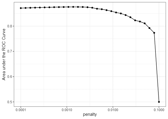
penaltyは小さいほうがよさそうですね。
縦が0.5になると、ほぼ予測できていないことになります。
BESTを選びます
top_models <-
lr_res %>%
show_best(metric = "roc_auc", n = 15) %>%
arrange(penalty)

top_models
#> # A tibble: 15 × 7
#>     penalty .metric .estimator  mean     n std_err .config
#>       <dbl> <chr>   <chr>      <dbl> <int>   <dbl> <chr>
#>  1 0.000127 roc_auc binary     0.872     1      NA Preprocessor1_Model02
#>  2 0.000161 roc_auc binary     0.872     1      NA Preprocessor1_Model03
#>  3 0.000204 roc_auc binary     0.873     1      NA Preprocessor1_Model04
#>  4 0.000259 roc_auc binary     0.873     1      NA Preprocessor1_Model05
#>  5 0.000329 roc_auc binary     0.874     1      NA Preprocessor1_Model06
#>  6 0.000418 roc_auc binary     0.874     1      NA Preprocessor1_Model07
#>  7 0.000530 roc_auc binary     0.875     1      NA Preprocessor1_Model08
#>  8 0.000672 roc_auc binary     0.875     1      NA Preprocessor1_Model09
#>  9 0.000853 roc_auc binary     0.876     1      NA Preprocessor1_Model10
#> 10 0.00108  roc_auc binary     0.876     1      NA Preprocessor1_Model11
#> 11 0.00137  roc_auc binary     0.876     1      NA Preprocessor1_Model12
#> 12 0.00174  roc_auc binary     0.876     1      NA Preprocessor1_Model13
#> 13 0.00221  roc_auc binary     0.876     1      NA Preprocessor1_Model14
#> 14 0.00281  roc_auc binary     0.875     1      NA Preprocessor1_Model15
#> 15 0.00356  roc_auc binary     0.873     1      NA Preprocessor1_Model16
ただし、モデルの性能が低下し始める地点に近いx軸上でペナルティ値を選択したいかもしれません。
性能がほぼ同じであれば、より高いペナルティ値を選択したいと考えるでしょう。この値を選択して、検証セットのROC曲線を可視化しましょう。
lr_best <-
lr_res %>%
collect_metrics() %>%
arrange(penalty) %>%
slice(12)

lr_best
#> # A tibble: 1 × 7
#>   penalty .metric .estimator  mean     n std_err .config
#>     <dbl> <chr>   <chr>      <dbl> <int>   <dbl> <chr>
#> 1 0.00137 roc_auc binary     0.876     1      NA Preprocessor1_Model12
lr_auc <-
lr_res %>%
collect_predictions(parameters = lr_best) %>%
roc_curve(children, .pred_children) %>%
mutate(model = "Logistic Regression")autoplot(lr_auc)
次のステップとして、木ベースのアンサンブル法を使用して生成される非常に非線形なモデルを考慮することができます。
2つ目のモデル:木ベースのアンサンブル
ランダムフォレストを試します。ただ、tuneの計算コストが高く時間がかかります。そのようなときは、以下のように並列処理ができます。
cores <- parallel::detectCores()

cores
#> [1] 10 ※CPUのコアが10個あるPCということ
※今回は並列処理を実行しないので省略します。
rf_mod <-
rand_forest(mtry = tune(), min_n = tune(), trees = 1000) %>%
set_engine("ranger", num.threads = cores) %>%
set_mode("classification")
※ハイパラの補足
mtry
内容: mtryは、各決定木の分岐ごとに考慮する変数の数を指定します。デフォルトでは、ランダムフォレストはすべての予測変数のうちランダムに選ばれたサブセットの中から最適な分割を選びます。
目的: モデルのバリアンス(過剰適合)とバイアス(適合不足)を調整します。小さなmtryはバリアンスを減少させ、バイアスを増加させる可能性があり、大きなmtryはその逆です。
min_n
内容: min_nは、各ノードがさらに分割されるために必要な最小のデータポイント数を指定します。このパラメータは、決定木の深さと複雑さを制御します。
目的: モデルの複雑さを管理し、過剰適合を防ぎます。小さなmin_nは非常に細かい分割を許可し、木が深くなる傾向があります。一方、大きなmin_nは木を浅くし、過剰適合を防ぐのに役立ちます。
前処理
rf_recipe <-
recipe(children ~ ., data = hotel_other) %>%
step_date(arrival_date) %>%
step_holiday(arrival_date) %>%
step_rm(arrival_date)
ワークフロー
rf_workflow <-
workflow() %>%
add_model(rf_mod) %>%
add_recipe(rf_recipe)
TRAINとTUNE
rf_mod
#> Random Forest Model Specification (classification)
#>
#> Main Arguments:
#>   mtry = tune()
#>   trees = 1000
#>   min_n = tune()
#>
#> Engine-Specific Arguments:
#>   num.threads = cores
#>
#> Computational engine: ranger
extract_parameter_set_dials(rf_mod)
#> Collection of 2 parameters for tuning
#>
#> identifier type object
#> mtry mtry nparam[?]
#> min_n min_n nparam[+]
#>
#> Model parameters needing finalization:
#> # Randomly Selected Predictors ('mtry')
#>
#> See `?dials::finalize` or `?dials::update.parameters` for more information.set.seed(345)
rf_res <-
rf_workflow %>%
tune_grid(val_set,
grid = 25,
control = control_grid(save_pred = TRUE),
metrics = metric_set(roc_auc))
#> i Creating pre-processing data to finalize unknown parameter: mtrygrid = 25で25個の候補からTUNEしています。
一番いいものを表示します。
rf_res %>%
show_best(metric = "roc_auc")

#> # A tibble: 5 × 8
#>    mtry min_n .metric .estimator  mean     n std_err .config
#>   <int> <int> <chr>   <chr>      <dbl> <int>   <dbl> <chr>
#> 1     8     7 roc_auc binary     0.926     1      NA Preprocessor1_Model13
#> 2    12     7 roc_auc binary     0.926     1      NA Preprocessor1_Model01
#> 3    13     4 roc_auc binary     0.925     1      NA Preprocessor1_Model05
#> 4     9    12 roc_auc binary     0.924     1      NA Preprocessor1_Model19
#> 5     6    18 roc_auc binary     0.924     1      NA Preprocessor1_Model24
ロジスティック回帰では、ROC AUCは0.876だったので、すでにそれを超えています。※数値が1に近いほうが良いと判断します。
autoplot(rf_res)
rf_best <-
rf_res %>%
select_best(metric = "roc_auc")

rf_best
#> # A tibble: 1 × 3
#>    mtry min_n .config
#>   <int> <int> <chr>
#> 1 8 7 Preprocessor1_Model13ROC曲線をプロットするために必要なデータを計算するには、collect_predictions()を使用します。これは、control_grid(save_pred = TRUE)を使用してチューニングした後にのみ可能です。出力には、子供を含むか含まないかを予測するクラス確率を保持する2つの列が表示されます。
rf_res %>%
collect_predictions()

#> # A tibble: 187,500 × 8
#>    .pred_children .pred_none id          .row  mtry min_n children .config
#>             <dbl>      <dbl> <chr>      <int> <int> <int> <fct>    <chr>
#>  1        0.152        0.848 validation    13    12     7 none     Preprocessor…
#>  2        0.0302       0.970 validation    20    12     7 none     Preprocessor…
#>  3        0.513        0.487 validation    22    12     7 children Preprocessor…
#>  4        0.0103       0.990 validation    23    12     7 none     Preprocessor…
#>  5        0.0111       0.989 validation    31    12     7 none     Preprocessor…
#>  6        0            1     validation    38    12     7 none     Preprocessor…
#>  7        0            1     validation    39    12     7 none     Preprocessor…
#>  8        0.00325      0.997 validation    50    12     7 none     Preprocessor…
#>  9        0.0241       0.976 validation    54    12     7 none     Preprocessor…
#> 10        0.0441       0.956 validation    57    12     7 children Preprocessor…
#> # ℹ 187,490 more rows
rf_auc <-
rf_res %>%
collect_predictions(parameters = rf_best) %>%
roc_curve(children, .pred_children) %>%
mutate(model = "Random Forest")bind_rows(rf_auc, lr_auc) %>%
ggplot(aes(x = 1 - specificity, y = sensitivity, col = model)) +
geom_path(lwd = 1.5, alpha = 0.8) + geom_abline(lty = 3) + coord_equal() +
scale_color_viridis_d(option = "plasma", end = .6)
最終FIT
TRAIN全体で再度モデルの学習を行います。
importance = "impurity" を追加します。これにより、この最後のモデルに対して変数重要度スコアが提供され、どの予測子がモデルの性能に寄与しているかの洞察が得られます。
the last model
last_rf_mod <-
rand_forest(mtry = 8, min_n = 7, trees = 1000) %>%
set_engine("ranger", num.threads = cores, importance = "impurity") %>%
set_mode("classification")
the last workflow
last_rf_workflow <-
rf_workflow %>%
update_model(last_rf_mod)
the last fit
set.seed(345)
last_rf_fit <-
last_rf_workflow %>%
last_fit(splits)
last_rf_fit
#> # Resampling results
#> # Manual resampling
#> # A tibble: 1 × 6
#> splits id .metrics .notes .predictions .workflow
#> <list> <chr> <list> <list> <list> <list>
#> 1 <split [37500/12500]> train/test sp… <tibble> <tibble> <tibble> <workflow>last_rf_fit %>%
collect_metrics()
#> # A tibble: 3 × 4
#> .metric .estimator .estimate .config
#> <chr> <chr> <dbl> <chr>
#> 1 accuracy binary 0.946 Preprocessor1_Model1
#> 2 roc_auc binary 0.923 Preprocessor1_Model1
#> 3 brier_class binary 0.0423 Preprocessor1_Model1どの変数が予測に効いているかを可視化します。
last_rf_fit %>%
extract_fit_parsnip() %>%
vip(num_features = 20)
重要な変数は以下の通り
部屋の1日あたりの費用
予約された部屋のタイプ
予約の作成日から到着日までの時間
最終的に割り当てられた部屋のタイプ
最後のROC曲線の生成
最後に、ROC曲線を生成して視覚化しましょう。予測するイベントが children 要因の最初のレベル(「子供がいる」)であるため、roc_curve() に適切なクラス確率 .pred_children を提供します。
last_rf_fit %>%
collect_predictions() %>%
roc_curve(children, .pred_children) %>%
autoplot()
後は予測するのみ!
ここからはチュートリアルに書いていませんが、
testという結果がわからないデータがあるなら以下のコードで予測ができます。
predict(last_rf_fit,test)END
この記事が気に入ったらサポートをしてみませんか?