Pythonライブラリ(ブラックボックス最適化/ハイパーパラメータ調整):Optuna

1.概要
機械学習モデルでは人間が手動設定する必要があるパラメータがあり、ハイパーパラメータと呼ばれます。ブラックボックス最適化ではハイパーパラメータに関する試行錯誤を自動化し、最適解を自動的に発見してくれます。オープンソースのフレームワークは下記がありますが、本記事ではOptunaを紹介します。
Optuna(開発:Preferred Networks)
gpyopt(開発:Machine Learning group of the University of Sheffield)
Optunaの詳細を学びたい方は(Pythonコードがある程度読める+最低限の数学・統計知識がある前提で)公式書である「Optunaによるブラックボックス最適化」がオススメです。
1-1.ハイパーパラメータとは
ハイパーパラメータとは機械学習モデルにおいて人間が手動で調整する必要があるパラメータです。詳細は下記記事に記載してます。
1-2.環境構築
optunaは下記実施するだけで使用可能です。ライブラリとして使用する場合は”import optuna”で読み込みます。
[Terminal]
pip install optuna2.Optunaのアルゴリズム
2-1.Optunaの特徴
Optunaには下記のような特徴があります。
ベイズ最適化の中でも新しい手法であるTPE(Tree-structured Parzen Estimator )というアルゴリズムを使用している。
並列処理が可能であり、結果をDatabaseに保存することで途中再開も可能
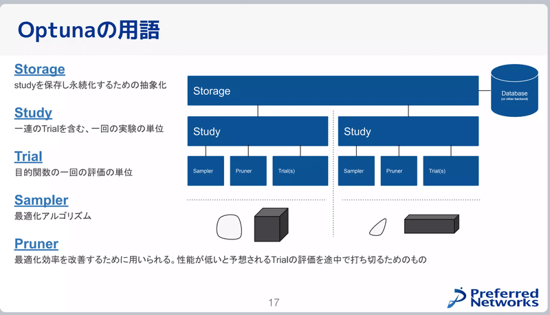
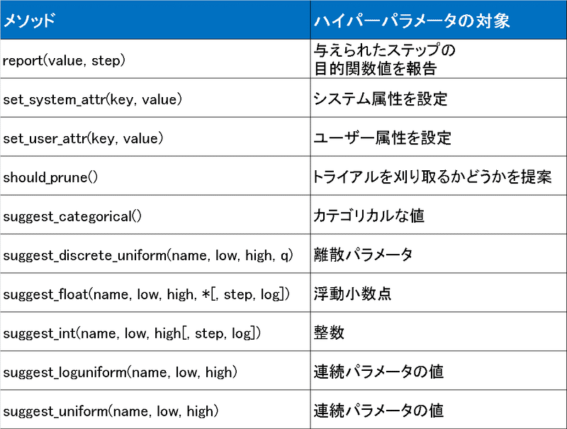
2-1.Optunaの用語
Optunaの用語は下記の通りです(出典:Optuna V3の全て )。
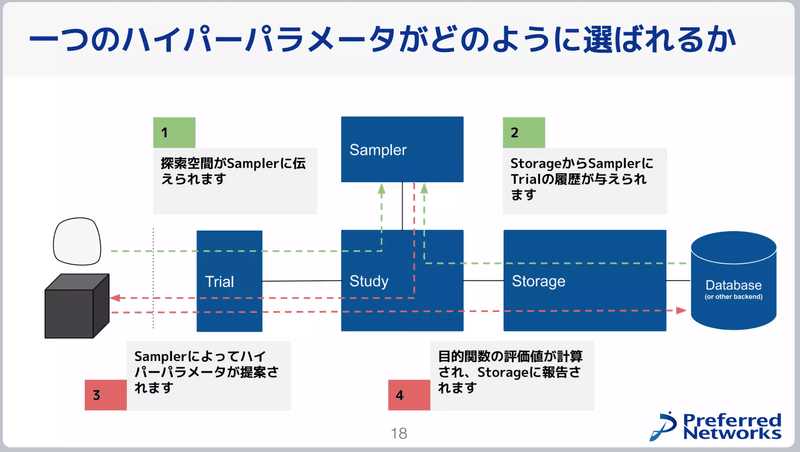
シンプルなOptunaの使用方法は下記の通りです。
目的関数(損失関数)を決める
trialオブジェクトを使用してハイパーパラメータの探索範囲を設定
"optuna.create_study()"でstudyオブジェクトを作成
”study.optimize”メソッドで最適化
3.Optunaの使い方(シンプル編)
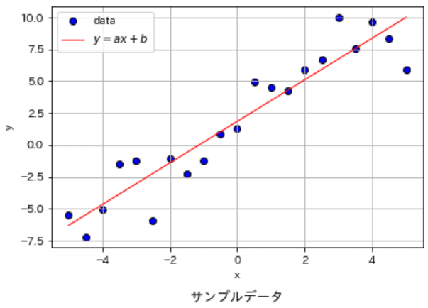
Optunaの使用方法は癖がある(と個人的に感じる)ため、まずは最もシンプルな例として単回帰モデルのパラメータ(傾き$${a}$$, 切片$${b}$$)の最適化を実施します。データは適当に作成しており解析解は$${a=1.63, b=1.84}$$となります。
$$
y=ax+b
$$
[IN]
import numpy as np
import pandas as pd
import matplotlib.pyplot as plt
import seaborn as sns
import japanize_matplotlib
from typing import List, Tuple, Dict, Optional
from mpl_toolkits.mplot3d import Axes3D
import os
import optuna

def make_outputdir(dirname: str='Output'):
    if not os.path.exists(dirname):
        os.makedirs(dirname)

def MeanSquaredError(label, y_pred):
    return np.mean((label - y_pred) ** 2)

def plot_data(ax, x, y, figtype, label, title=None, verbose=False):
    if figtype == 'scatter':
        ax.scatter(x, y, c='blue', edgecolors='k', label=label)
    elif figtype == 'line':
        ax.plot(x, y, c='red', lw=1.0, label=label)
    else:
        raise ValueError('figtype must be "scatter" or "line"')
    ax.set_xlabel('x')
    ax.set_ylabel('y')
    if title is not None:
        ax.set_title(title, y=-0.25)
    if verbose:
        ax.grid()
        ax.legend()

#フォルダ作成
make_outputdir(dirname='Output') #出力フォルダ作成

#データ作成
np.random.seed(0)
x = np.linspace(-5, 5, 21)
y = 2 * x + 1 + np.random.randn(21)*2
pd.options.display.float_format = '{:.2f}'.format #Pandasの表示桁数を指定
display(pd.DataFrame({'x': x, 'y': y}).T)

#解析解の確認
slope_calc, intercept_calc = np.polyfit(x, y, 1)
print(f'解析解 傾き:{slope_calc:.3f} 切片:{intercept_calc:.3f}')
print(f'解析解のMSE:{MeanSquaredError(y, slope_calc * x + intercept_calc):.3f}')
fig, ax = plt.subplots(1, 1, figsize=(6, 4))
plot_data(ax, x, y, figtype='scatter', label='data', verbose=False)
plot_data(ax, x, slope_calc * x + intercept_calc, label=r'$y=ax+b$',  figtype='line', verbose=True, title='サンプルデータ')
plt.show()
[OUT]
解析解 傾き:1.631 切片:1.841
解析解のMSE:3.274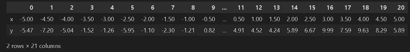
3-1.シンプルなOptunaのコード
Optunaのプロセスは下記の通りであり、それを表現したコードを示します。
objective(trial)関数の作成:目的関数からパラメータを学習するための関数を作成します。慣例として"def objective(trial):"を使用します。
パラメータの探索範囲を指定:”trial_suggest_”を用いて最適化したいパラメータの探索範囲を指定して変数に格納します。なおパラメータの型による"suggest_"の後ろの文字が変化します。
目的関数を定義:誤差関数や尤度関数のように機械学習モデルを評価するための指標を定義します。変数はsuggest_で定義したものを使用します。今回は目的関数として$${\text{MSE} = \frac{1}{n}\sum_{i=1}^{n}(y_i - \hat{y}_i)^2}$$を使用しました。
最適化を実行:”optuna.create_study()”で目的関数を最適化します。今回の目的関数:MSEは誤差のため引数の"direction"でMSEを最小化します。最適化の実行は”study.optimize(objective, n_trials)”となります。
最適化後のパラメータ/目的関数の確認:実行後の結果はStudyオブジェクトに格納されます。最適パラメータは”study.best_params”, その時の目的関数の値は"study.best_value"に格納されます(今回はMSEのため最適化は最小値が出力されます)。
[IN]
import optuna

def objective(trial):
    a = trial.suggest_uniform('a', -5, 5)
    b = trial.suggest_uniform('b', -5, 5)

    y_pred = a * x + b #予測値
    mean_squared_error = np.mean((y - y_pred)**2) #MSE
    return mean_squared_error

#Optunaで最適化
study = optuna.create_study(direction='minimize') #目的関数(MSE)を最小化
study.optimize(objective, n_trials=100)

#結果表示
print(f'最適パラメータ:{study.best_params}')
print(f'目的関数の最小値:{study.best_value:.3f}')[OUT]
[32m[I 2023-04-11 21:40:34,674][0m A new study created in memory with name: no-name-5b50fd9f-e66b-48b1-a6c5-ac72974e9e38[0m
[32m[I 2023-04-11 21:40:34,677][0m Trial 0 finished with value: 31.24606129440494 and parameters: {'a': 2.740411495836157, 'b': -2.2440713900375595}. Best is trial 0 with value: 31.24606129440494.[0m
[32m[I 2023-04-11 21:40:34,677][0m Trial 1 finished with value: 17.083097651645907 and parameters: {'a': 0.6025837803677483, 'b': -0.18681922145120033}. Best is trial 1 with value: 17.083097651645907.[0m
[32m[I 2023-04-11 21:40:34,678][0m Trial 2 finished with value: 116.59026196627032 and parameters: {'a': 4.617505723440672, 'b': -3.776383985783788}. Best is trial 1 with value: 17.083097651645907.[0m
[32m[I 2023-04-11 21:40:34,680][0m Trial 3 finished with value: 88.75548905007302 and parameters: {'a': -1.3285285799931303, 'b': 4.119562477448429}. Best is trial 1 with value: 17.083097651645907.[0m
[32m[I 2023-04-11 21:40:34,681][0m Trial 4 finished with value: 55.960898602378336 and parameters: {'a': 0.21065174603605374, 'b': -4.006185974428252}. Best is trial 1 with value: 17.083097651645907.[0m
[32m[I 2023-04-11 21:40:35,233][0m Trial 93 finished with value: 4.219703411926963 and parameters: {'a': 1.9267188259131942, 'b': 2.22091713434412}. Best is trial 72 with value: 3.3335859492255198.[0m
[32m[I 2023-04-11 21:40:35,240][0m Trial 94 finished with value: 4.6186770547205445 and parameters: {'a': 1.251034223433133, 'b': 1.696862386187241}. Best is trial 72 with value: 3.3335859492255198.[0m
[32m[I 2023-04-11 21:40:35,247][0m Trial 95 finished with value: 3.4326800143379153 and parameters: {'a': 1.6670047583525995, 'b': 1.4583384681846758}. Best is trial 72 with value: 3.3335859492255198.[0m
[32m[I 2023-04-11 21:40:35,253][0m Trial 96 finished with value: 4.319646142677267 and parameters: {'a': 1.7775527193133824, 'b': 0.9200555042121783}. Best is trial 72 with value: 3.3335859492255198.[0m
[32m[I 2023-04-11 21:40:35,260][0m Trial 97 finished with value: 11.700132204557079 and parameters: {'a': 2.43288862123923, 'b': 0.2500592904396547}. Best is trial 72 with value: 3.3335859492255198.[0m
[32m[I 2023-04-11 21:40:35,267][0m Trial 98 finished with value: 11.387679674773812 and parameters: {'a': 1.0248514499822616, 'b': -0.3370377919109451}. Best is trial 72 with value: 3.3335859492255198.[0m
[32m[I 2023-04-11 21:40:35,273][0m Trial 99 finished with value: 3.734963718970038 and parameters: {'a': 1.4641476694109135, 'b': 1.3879726001755393}. Best is trial 72 with value: 3.3335859492255198.[0m
最適パラメータ:{'a': 1.636239160182889, 'b': 2.084578843362393}
目的関数の最小値:3.334Studyオブジェクト内のメソッドは下記の通りです。”study.trials”でTrialの情報が確認できます。
[IN]
print(f'studyのメソッド一覧:{[i for i in dir(study) if not i.startswith("_")]}')

print(f'stydy.trialsの情報 型:{type(study.trials)}, 要素数:{len(study.trials)}, 要素の型:{type(study.trials[0])}')
print(study.trials[0]) #最初の試行
print(study.trials[-1]) #最後の試行


[OUT]
studyのメソッド一覧:['add_trial', 'add_trials', 'ask', 'best_params', 'best_trial',
'best_trials', 'best_value', 'direction', 'directions', 'enqueue_trial', 'get_trials',
'optimize', 'pruner', 'sampler', 'set_system_attr', 'set_user_attr', 'stop', 'study_name',
'system_attrs', 'tell', 'trials', 'trials_dataframe', 'user_attrs']


stydy.trialsの情報 型:<class 'list'>, 要素数:100, 要素の型:<class 'optuna.trial._frozen.FrozenTrial'>
FrozenTrial(number=0, values=[3.868117145051878], datetime_start=datetime.datetime(2023, 4, 11, 22, 58, 20, 578517), datetime_complete=datetime.datetime(2023, 4, 11, 22, 58, 20, 578517), params={'a': 1.400220237414815, 'b': 4.700664019301534}, distributions={'a': UniformDistribution(high=5.0, low=0.0), 'b': UniformDistribution(high=5.0, low=0.0)}, user_attrs={}, system_attrs={}, intermediate_values={}, trial_id=0, state=TrialState.COMPLETE, value=None)
FrozenTrial(number=99, values=[0.34590910718523915], datetime_start=datetime.datetime(2023, 4, 11, 22, 58, 21, 185516), datetime_complete=datetime.datetime(2023, 4, 11, 22, 58, 21, 191516), params={'a': 2.865062897082082, 'b': 2.4712694481297226}, distributions={'a': UniformDistribution(high=5.0, low=0.0), 'b': UniformDistribution(high=5.0, low=0.0)}, user_attrs={}, system_attrs={}, intermediate_values={}, trial_id=99, state=TrialState.COMPLETE, value=None)
3-2.動作を可視化1:MSEの確認
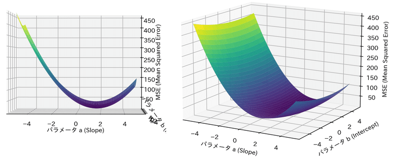
Optunaの最適化がどのように動いているか確認します。まずは目的関数のMSEがどのような形状か3Dプロットと等高線図で確認しました。
形状はお椀型であり極小点(谷底)が1点存在することが確認できます。
[IN]
%matplotlib qt
import numpy as np
import optuna
import matplotlib.pyplot as plt
from mpl_toolkits.mplot3d import Axes3D


# 等高線プロット
a_range = np.linspace(-5, 5, 100)
b_range = np.linspace(-5, 5, 100)
a_grid, b_grid = np.meshgrid(a_range, b_range)
#Z軸の値:MSE(Mean Squared Error)
mse_grid = np.array([
    np.mean((y - (a * x + b)) ** 2) for a, b in zip(a_grid.ravel(), b_grid.ravel())
]).reshape(a_grid.shape)

print(f'3次元プロット用形状確認:x={a_grid.shape}, y={b_grid.shape}, z={mse_grid.shape}:')

# 2次元プロット:等高線(塗りつぶし)
fig = plt.figure(figsize=(8, 6), facecolor="white")
plt.contourf(a_grid, b_grid, mse_grid, levels=20, cmap="coolwarm")
plt.colorbar()
plt.xlabel("パラメータ a (Slope)")
plt.ylabel("パラメータ b (Intercept)")
plt.xticks(np.arange(-5, 5.1, 1)), plt.yticks(np.arange(-5, 5.1, 1))

# 解析解をプロット
plt.plot(slope_calc, intercept_calc, marker="x", color="red", label="解析解", markersize=12)
plt.text(slope_calc, intercept_calc-1, f'(a={slope_calc:.2f}, b={intercept_calc:.2f})', color="red", fontsize=12)

# Optunaでの最適解をプロット
plt.plot(study.best_params["a"], study.best_params["b"], marker="^", color="yellow", label="Optunaで計算", markersize=10)
plt.text(study.best_params["a"], study.best_params["b"]+1, f'(a={study.best_params["a"]:.2f}, b={study.best_params["b"]:.2f})', color="yellow", fontsize=12)
plt.legend(loc="upper left")
plt.savefig("Output/2d_contour.png")
plt.show()

# 3次元プロット
fig = plt.figure(figsize=(8, 6), facecolor="white")
ax = fig.add_subplot(111, projection="3d")
ax.plot_surface(a_grid, b_grid, mse_grid, cmap="viridis")
ax.set_xlabel("パラメータ a (Slope)")
ax.set_ylabel("パラメータ b (Intercept)")
ax.set_zlabel("MSE (Mean Squared Error)")
plt.show()

[OUT]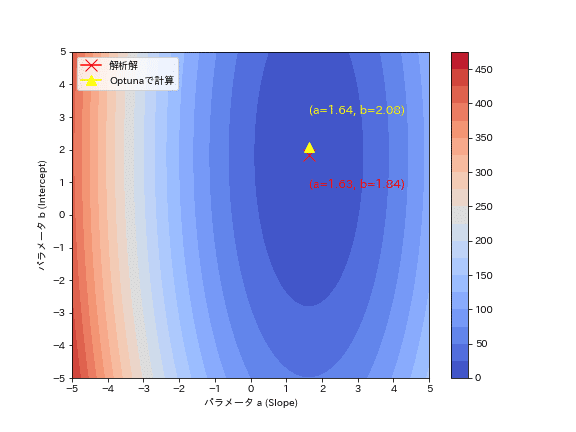
3-3.動作を可視化2:MSEの確認
Optunaの試行結果からパラメータがどのように最適化されているかを確認しました。結果としてジグザグしながら最適解に近づいていることが分かります。勾配降下法のように必ず谷底(勾配と反対方向)に移動しているわけではないことが確認できます。
[IN]
from matplotlib.animation import FuncAnimation

fig, ax = plt.subplots(figsize=(8, 6), facecolor="white")

# 等高線を描画
contourf = ax.contourf(a_grid, b_grid, mse_grid, levels=20, cmap="coolwarm")
fig.colorbar(contourf)

# 解析解をプロット
ax.plot(slope_calc, intercept_calc, marker="x", color="r", label="解析解", markersize=12)

# Optunaでの最適解をプロット
optuna_path, = ax.plot([], [], marker="^", color="yellow", label="Optunaで計算", markersize=4, lw=0.3)

# trial回数とx, yの値を表示するテキストボックス
text_box = ax.text(0.05, 0.95, "", transform=ax.transAxes, fontsize=10,
                   verticalalignment="top", bbox=dict(facecolor="w", alpha=0.5))

ax.set_xlabel("パラメータa (Slope)")
ax.set_ylabel("パラメータb (Intercept)")
ax.legend(loc="lower left")

# 初期化関数
def init():
    optuna_path.set_data([], [])
    text_box.set_text("") # テキストボックスを空にする
    return optuna_path, text_box

# アニメーションの更新関数
def update(frame):
    a_values = [t.params["a"] for t in study.trials[:frame+1]]
    b_values = [t.params["b"] for t in study.trials[:frame+1]]

    optuna_path.set_data(a_values, b_values)

    text_box.set_text(f"Trial: {frame+1}\na: {a_values[-1]:.2f}\nb: {b_values[-1]:.2f}")

    return optuna_path, text_box

# アニメーションの作成
ani = FuncAnimation(fig, update, frames=len(study.trials), init_func=init, blit=True, interval=400)

# GIFファイルに保存
ani.save("Output/optuna_animation.gif", writer="imagemagick", fps=5)
plt.show()

[OUT]
3-4.簡単な機械学習モデルで実装
実際に簡単な機械学習モデルを使用して最適化してみます。お馴染みのIrisデータセットを決定木モデルを使用して①ハイパラを手動で適当に設定、②Optunaで探索 した結果を比較します。結果としてOptunaで最適化することで精度が改善されることを確認できました。
[IN]
from sklearn import datasets
from sklearn.tree import DecisionTreeClassifier
from sklearn.model_selection import cross_val_score
from sklearn.model_selection import train_test_split

#Irisデータセットの読み込み
iris = datasets.load_iris()
data, target = iris.data, iris.target

#データセットの分か
X_train, X_test, y_train, y_test = train_test_split(data, target, test_size=0.2, random_state=0)

#通常通り学習
tree_clf = DecisionTreeClassifier(random_state=0, max_depth=3, min_samples_leaf=2)
tree_clf.fit(X_train, y_train)
y_pred = tree_clf.predict(X_test)
acc_train, acc_test = tree_clf.score(X_train, y_train), tree_clf.score(X_test, y_test)
print(f'精度 訓練:{acc_train:.3f} テスト:{acc_test:.3f}')

#Optunaでパラメータ探索

def objective_tree(trial):
    max_depth = trial.suggest_int('max_depth', 1, 10)
    min_samples_leaf = trial.suggest_int('min_samples_leaf', 1, 10)

    tree_clf = DecisionTreeClassifier(random_state=0, max_depth=max_depth, min_samples_leaf=min_samples_leaf)
    tree_clf.fit(X_train, y_train)
    acc_test = tree_clf.score(X_test, y_test)
    return acc_test

study = optuna.create_study(direction='maximize')
study.optimize(objective_tree, n_trials=100)
print(f'最適なパラメータ:{study.best_params}')
print(f'最適な精度:{study.best_value:.3f}')[OUT]
精度 訓練:0.967 テスト:0.967
[I 2023-04-15 10:31:45,345] A new study created in memory with name: no-name-f38633bf-253f-4763-8492-b747d4ed80ee
[I 2023-04-15 10:31:45,348] Trial 0 finished with value: 0.5666666666666667 and parameters: {'max_depth': 1, 'min_samples_leaf': 6}. Best is trial 0 with value: 0.5666666666666667.
[I 2023-04-15 10:31:45,350] Trial 1 finished with value: 0.9666666666666667 and parameters: {'max_depth': 6, 'min_samples_leaf': 10}. Best is trial 1 with value: 0.9666666666666667.
[I 2023-04-15 10:31:45,351] Trial 2 finished with value: 0.9666666666666667 and parameters: {'max_depth': 8, 'min_samples_leaf': 8}. Best is trial 1 with value: 0.9666666666666667.
・・・・・
[I 2023-04-15 10:31:46,011] Trial 97 finished with value: 1.0 and parameters: {'max_depth': 8, 'min_samples_leaf': 4}. Best is trial 3 with value: 1.0.
[I 2023-04-15 10:31:46,020] Trial 98 finished with value: 1.0 and parameters: {'max_depth': 8, 'min_samples_leaf': 4}. Best is trial 3 with value: 1.0.
[I 2023-04-15 10:31:46,028] Trial 99 finished with value: 1.0 and parameters: {'max_depth': 7, 'min_samples_leaf': 3}. Best is trial 3 with value: 1.0.
最適なパラメータ:{'max_depth': 9, 'min_samples_leaf': 3}
最適な精度:1.0004.Optuna基礎:基本処理
前章でも紹介した内容も含めてOptunaの基本的なメソッドを紹介します。
4-1.目的関数の定義:objective(trial)
Optunaで最適化を実行するための目的関数を定義します。慣例として”def objective(trial)”を使用します。
[IN]
def func1(x, a:float):
    return (x-a)**2


def objective(trial):
    x = trial.suggest_uniform('x', -5, 5) #suggest_ は変数に格納する
    y = func1(x, 2) #suggest_ で格納した変数を使って関数を実行
    return y

study = optuna.create_study(direction='minimize')
study.optimize(objective, n_trials=20)
print(study.best_params, study.best_value)
[OUT]
詳細は後述4-2.パラメータの範囲選定:trial.suggest_
ハイパーパラメータの型と探索範囲指定に"trial.suggest_"を使用します。
ポイントとして、1.探索したい変数の対象に合わせてメソッドを選定、2.suggest_()を変数に格納してその変数を目的変数に渡す ことです。下記では$${(x-2)^2}$$をx軸で最小化した結果です。
[IN]
def func1(x, a:float):
    return (x-a)**2


def objective(trial):
    x = trial.suggest_uniform('x', -5, 5) #suggest_ は変数に格納する
    y = func1(x, 2) #suggest_ で格納した変数を使って関数を実行
    return y

study = optuna.create_study(direction='minimize')
study.optimize(objective, n_trials=20)
print(study.best_params, study.best_value)[OUT]
{'x': 2.2148486123090523} 0.046159926211125454-3.Studyの作成:optuna.create_study()
"optuna.create_study()"を実行することでStudyオブジェクトを作成します。”create_study()”メソッドの中で使用頻度の高い引数のみ紹介します。なお1つのDataBase(DB)内に複数のStudyを作成できますが、同一DB内ではStudy名は一意である必要があります。
direction:目的関数を最適化への目標("minimize", "maximize"など)
study__name:DBに任意のStudyを保存可
storage:SQLITEでDBの保存ファイルを作成
sampler:ブラックボックス最適化アルゴリズムを選択
[API]
optuna.create_study(*, storage=None, sampler=None, pruner=None, study_name=None,
direction=None, load_if_exists=False, directions=None)参考例として単回帰モデルを最小化後にファイルを作成しました。
[IN]
#データ作成
np.random.seed(0)
x = np.linspace(-5, 5, 21)
y = 2 * x + 1 + np.random.randn(21)*2

def objective(trial):
    a = trial.suggest_uniform('a', -5, 5)
    b = trial.suggest_uniform('b', -5, 5)

    y_pred = a * x + b #予測値
    mean_squared_error = np.mean((y - y_pred)**2) #MSE
    return mean_squared_error

#Optunaで最適化+DBに保存
study = optuna.create_study(direction='minimize',
                            study_name='Optunaで単回帰分析',
                            storage='sqlite:///optuna_単回帰.db')
study.optimize(objective, n_trials=100)

[OUT]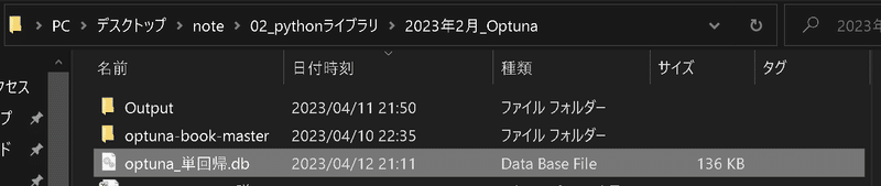
4-4.Studyの実行(最適化):study.optimize()
Studyの実行は”study.optimize()”で実行します。funcには目的関数の"objective"を渡し、"n_trial"にはTrial回数を指定します。
[API]
optimize(func, n_trials=None, timeout=None, n_jobs=1,
         catch=(), callbacks=None, gc_after_trial=False, show_progress_bar=False)
4-5.Studyの保存/再開:optuna.load_study()
前述の通りStudyの保存は"optuna.create_study(storage=<DB名>, study_name=<Studyの名前>)で実行できます。
DBから保存したStudyの読み込みは”optuna.load_study()”を使用します。DBには複数のStudyが存在できるため、DBファイルだけでなくStudy名の指定も必須です。
[API]
optuna.study.load_study(*, study_name, storage, sampler=None, pruner=None)[IN]
study_restart = optuna.load_study(study_name='Optunaで単回帰分析',
storage='sqlite:///optuna_単回帰.db')
print(study_restart.study_name)
print(f'study.best_params: {study_restart.best_params}')
print(f'study.best_value: {study_restart.best_value}')[OUT]
Optunaで単回帰分析
study.best_params: {'a': 1.6750741649686536, 'b': 1.8128715603918766}
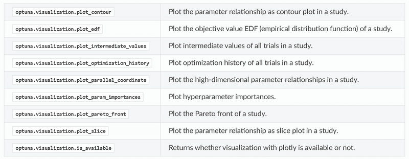
study.best_value: 3.29274366314269475.Optuna基礎:分析/可視化
Optunaでは最適化の結果がStudyに格納されており、最適化のデータ確認や可視化が可能です。
可視化に関しては”optuna.visualization”モジュールで使用でき、等高線図やトライアル履歴の表示などが可能です。
5-1.Studyオブジェクトの情報
Studyオブジェクトのメソッドや属性は下記の通りです。
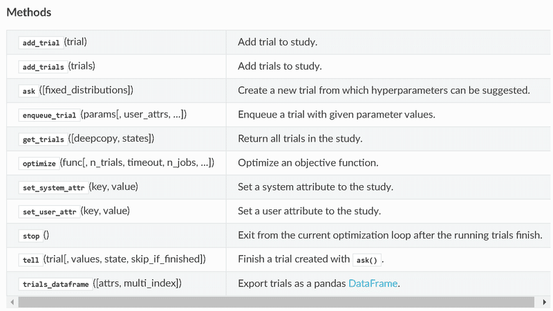
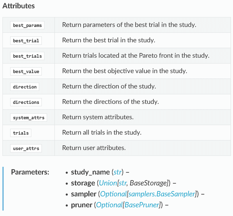
5-2.最適化の履歴表示:trials_dataframe()
最適化の履歴はStudyオブジェクトの"trials_dataframe()"メソッドよりDataFrame型として抽出可能です。データをソートすることで何回目の処理で最適化され、その時のパラメータがいくらかを確認できます。
[IN]
df_study = study.trials_dataframe()
display(df_study.head(3)) #Studyの詳細:先頭3行
display(df_study.tail(3)) #Studyの詳細:末尾3行

df_study.sort_values('value', ascending=True).head() #value(目的関数:MSE)が小さい順に並べ替え

[OUT]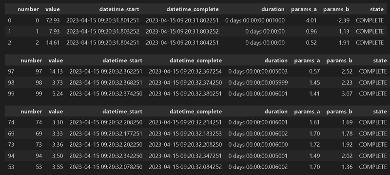
参考としてstate列の意味は公式に紹介されております。
5-3.パラメータの重要度:X_param_importance()
Optunaではハイパーパラメータ重要度の評価にfANOVAというアルゴリズムを用いて計算しています。数値および可視化はそれぞれ下記の通りです。
[IN]
# パラメータの重要度:OptunaはfANOVA
importances = optuna.importance.get_param_importances(
    study=study,
    params=['a', 'b'])

for k, v in importances.items():
    print(f'{k}: {v}')

[OUT]
a: 0.9909789972229721
b: 0.009021002777027947[IN]
optuna.visualization.plot_param_importances(
study=study,
params=['a', 'b']).show()
[OUT]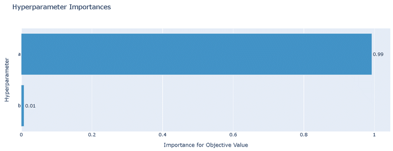
シンプルな結果ですが、下図の単回帰モデルでは切片より傾きの方が重要であることが確認できました。
5-4.等高線プロットによる可視化:plot_contour
"optuna.visualization.plot_contour()"によりハイパーパラメータと評価値の関係をより詳細に可視化できます。
本例では単回帰モデル$${y=ax+b}$$における傾き$${a}$$, 切片$${b}$$の等高線がプロットされており色が薄いほどよい(最小化されている)ことが分かります。また黒マーカーは各トライアルでのハイパラの値を示します。
[IN]
#等高線プロット
optuna.visualization.plot_contour(
    study=study,
    params=['a', 'b']).show()

[OUT]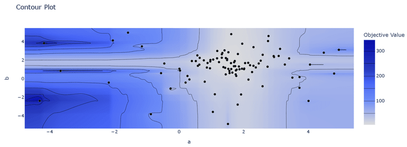
結果を見ると”a軸方向にグラデーションがあるためaが全体的に最適化パラメータに影響がある。bは1.8付近から外れると一気に目的関数が悪くなる”ことが確認できます。
5-5.トライアル履歴可視化:plot_optimization_history()
トライアル履歴可視化は"plot_optimization_history()"を使用します。
[IN]
optuna.visualization.plot_optimization_history(study=study).show()

[OUT]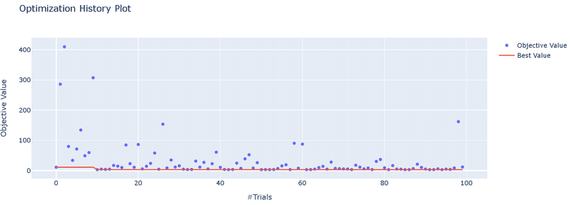
6.Optuna応用
6-1.多目的最適化/パレートフロント
Optunaでは複数の目的変数の最適化も可能です。前提として「Optunaは複数の目的間のトレードオフ(パレートフロント)の探索までを行い、最終的なパラメータは人が選択」する思想があるとのことです。
またOptunaの多目的最適化アルゴリズムは基本的に目的数が3以下を想定しているため、それより多い場合はできる限り目的数を3以下に下げるほうが性能がでます。
6-1-1.多目的最適化とは
目的関数が「1つ」だけの最適化を単目的最適化に対して、目的関数が複数ある最適化を多目的最適化と呼びます。例として2021年にSOTAを獲得した画像モデル"EfficientNetV2"では精度、モデルのサイズ、学習時間の3つの指標を多目的最適化することで発見されたモデルとなります。
単目的最適化における最適解は1つに対して、多目的最適化の場合にはトレードオフの関係が発生するため最適解は1つとは限りません。トレードオフが発生する中で最適解の集合を「パレート最適解」と呼びます。
http://www.iba.t.u-tokyo.ac.jp/iba/AI/MO.pdf
考え方の概要として「投資額」と「リターン」のデータを考えてみます。投資額が大きいほどリターンの絶対値も大きくなりますが割合としてはどこかで頭打ちになります。投資額は最小でリターンが最大となる点を探したいと思います。まずは最小化問題に変更するためリターンは逆数で考えます。
[IN]
def plot_data(ax, x, y, figtype, label, xlabel, ylabel, title=None, verbose=False):
    if figtype == 'scatter':
        ax.scatter(x, y, c='blue', edgecolors='k', label=label)
    elif figtype == 'line':
        ax.plot(x, y, c='red', lw=1.0, label=label)
    else:
        raise ValueError('figtype must be "scatter" or "line"')
    ax.set_xlabel(xlabel)
    ax.set_ylabel(ylabel)
    if title is not None:
        ax.set_title(title, y=-0.25)
    if verbose:
        ax.grid()
        ax.legend()

#データ作成
np.random.seed(5)
datas = np.random.rand(2, 11) # 2次元配列
invests, returnvalues = datas[0], datas[1]
inv_returnvalues = 1 / returnvalues

fig, ax = plt.subplots(1, 1, figsize=(6, 4))
plot_data(ax, invests, returnvalues, figtype='scatter', label='data', xlabel='投資額', ylabel='リターン', verbose=True)

fig, ax = plt.subplots(1, 1, figsize=(6, 4))
plot_data(ax, invests, 1/returnvalues, figtype='scatter', label='data', xlabel='投資額', ylabel=r'1/リターン', verbose=True)

[OUT]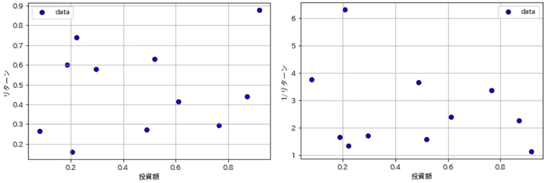
それぞれの点を比較した時、投資・リターンがともに劣っている点があることが確認できます($${投資額_A>投資額_B \cap\frac{1}{リターン_A}>\frac{1}{リターン_B}}$$となるため、特定の点より右上に存在しうる点が該当)。
つまりこれらは最適解にはなりえないため、それらを除外すると最適解の候補(非劣解)が得られます。
[IN]
import numpy as np
import matplotlib.pyplot as plt

colors_dict = {0: 'red', 1: 'blue', 2: 'green', 3: 'yellow', 4: 'black', 5: 'pink', 6: 'orange', 7: 'purple', 8: 'brown', 9: 'gray'}

#プロット図で指定した点の右上を塗りつぶす関数
def fill_dominated_area(optimal_investment, optimal_inv_returnrate, invests, inv_returnvalues, ax, color='gray', alpha=0.3):
    ax.fill_between(
        [optimal_investment, invests.max()], [optimal_inv_returnrate, optimal_inv_returnrate],
        [inv_returnvalues.max(), inv_returnvalues.max()],
        color=color, alpha=alpha
    )

#パレートフロントを求める関数
def is_pareto_efficient(datas: np.ndarray)->np.ndarray:
    is_efficient = np.ones(datas.shape[0], dtype=bool) #データ数だけTrueの配列を作成
    for i, c in enumerate(datas):
        if is_efficient[i]:
            is_efficient[is_efficient] = np.any(datas[is_efficient] <= c, axis=1) #抽出したデータ[投資額, 1/リターン]を全データ内で比較し、劣解をFalseにする
            is_efficient[i] = True
    return is_efficient

datasets = np.array([invests, inv_returnvalues]).T
display(datasets)
pareto_efficient = is_pareto_efficient(datasets)
print(pareto_efficient)

datasets_dominate = datasets[pareto_efficient] #非劣解のデータ
datasets_non_dominate = datasets[~pareto_efficient] #劣解のデータ
print(f'非劣解 データ数:{datasets_dominate.shape[0]}')
print(f'劣解 データ数:{datasets_non_dominate.shape[0]}')

#プロット
fig, ax = plt.subplots(1, 1, figsize=(8, 6), facecolor='w')
ax.scatter(datasets_dominate[:, 0], datasets_dominate[:, 1], color='r', label='非劣解')
ax.scatter(datasets_non_dominate[:, 0], datasets_non_dominate[:, 1], color='b', label='劣解')
for i, (x, y) in enumerate(zip(invests, inv_returnvalues)):
    ax.text(x, y, f'({x:.2f}, {y:.2f})', fontsize=9, ha='right', va='bottom' if i % 2 == 0 else 'top')

for i, (x, y) in enumerate(zip(invests[pareto_efficient], inv_returnvalues[pareto_efficient])):
    fill_dominated_area(x, y, invests, inv_returnvalues, color=colors_dict[i], alpha=0.3, ax=ax)

ax.set(xlabel='投資額', ylabel='1/リターン', title='パレート最適解',xticks=np.arange(0, 1.1, 0.1))
ax.legend(), ax.grid()
plt.show()
[OUT]
array([[0.22199317, 1.35420562],
[0.87073231, 2.26598482],
[0.20671916, 6.31672564],
[0.91861091, 1.13644496],
[0.48841119, 3.64848374],
[0.61174386, 2.41408851],
[0.76590786, 3.37746632],
[0.51841799, 1.59036137],
[0.2968005 , 1.7246202 ],
[0.18772123, 1.66686337],
[0.08074127, 3.76195666]])
[ True False False True False False False False False True True]
非劣解 データ数:4
劣解 データ数:7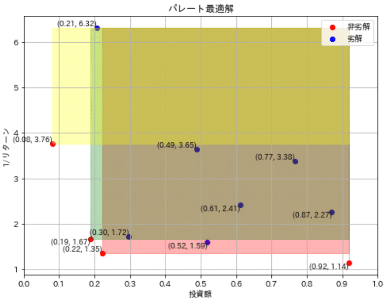
この候補の中で一番左下に存在するデータを抽出することで最適解を選定できます。今回はx軸とy軸の合計値が最小になる値で選定しました。非劣解は選定されているため、もし投資額に上限があるのであれば、上限を設定して最適解を選定したらよく、最終的な判断は解析者が設定可能です。
[IN]
pareto_invests = invests[pareto_efficient]
pareto_inv_returnvalues = inv_returnvalues[pareto_efficient]
print(pareto_invests + pareto_inv_returnvalues)

optimal_index = np.argmin(pareto_invests + pareto_inv_returnvalues)
optimal_investment = pareto_invests[optimal_index]
optimal_inv_returnrate = pareto_inv_returnvalues[optimal_index]
print(f'最適解 index: {optimal_index}, 投資額: {optimal_investment:.2f}, 1/リターン: {optimal_inv_returnrate:.2f}')

fig, ax = plt.subplots(1, 1, figsize=(8, 6), facecolor='w')
plot_data(ax, invests, inv_returnvalues, figtype='scatter', label='data', xlabel='投資額', ylabel=r'1/リターン', verbose=True)
ax.scatter(optimal_investment, optimal_inv_returnrate, color='green', marker='*', s=200, label='最適解')
ax.legend()
plt.show()

[OUT]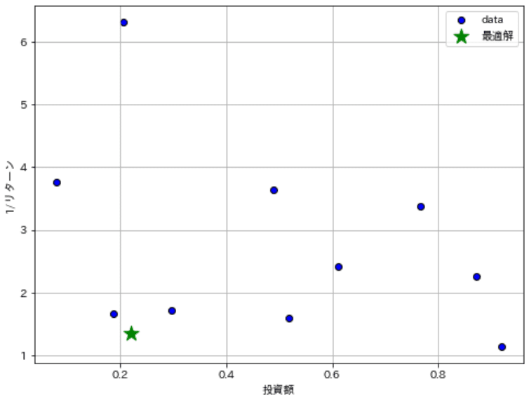
6-1-2.Optunaでの多目的最適化
サンプルデータは$${f_1(x)=(x-2)^2}$$, $${f_2(x)=(x-4)^2}$$を使用します。それぞれの最小値は$${(x_1,y_1)=(2,0)}$$, $${(x_2,y_2)=(4,0)}$$となり、片方を最適化すると片方が悪くなるトレードオフの関係にあります。
[IN]
def func1(x, a):
    return (x - a)**2

x = np.linspace(0, 10, 100)
y1, y2 = func1(x, 2), func1(x, 4)

fig, ax = plt.subplots()
ax.plot(x, y1, label=r'$(x - 2)^2$')
ax.plot(x, y2, label=r'$(x - 4)^2$')
ax.set(xlabel='x', ylabel='y', xticks=np.arange(0, 11, 1))
ax.legend(), ax.grid()
plt.show()

[OUT]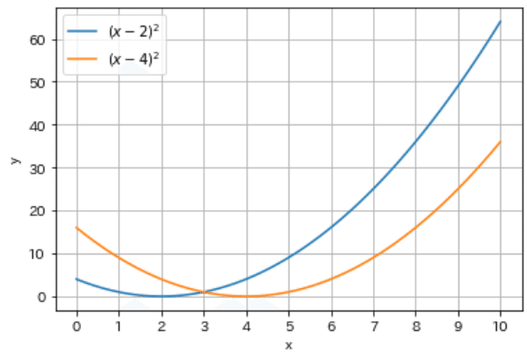
Optunaでの多目的最適化の記法は下記の通りです。
"def objective(trial)"の戻り値を複数指定
"optuna.create_study()"を"directions=[<条件1>, <条件2>・・]"に設定
最適解は”study.best_trials”で出力
[IN]
def objective(trial):
    x = trial.suggest_uniform('x', 0, 10)

    y1 = func1(x, 2)
    y2 = func1(x, 4)
    return y1, y2

study = optuna.create_study(
    directions=['minimize', 'minimize']
)

study.optimize(objective, n_trials=100)

for t in study.best_trials:
    print(f't.number: {t.number}, params: {t.params}, values: {t.values}')
[OUT]
t.number: 2, params: {'x': 3.3908476129855227}, values: [1.9344570825475265, 0.3710666306054355]
t.number: 11, params: {'x': 3.7736029181777986}, values: [3.1456673113688027, 0.051255638657608564]
t.number: 13, params: {'x': 3.091270523430615}, values: [1.1908713553085286, 0.8257892615860684]
t.number: 17, params: {'x': 2.5568008315996362}, values: [0.31002716607004643, 2.0828238396715015]
t.number: 19, params: {'x': 3.727244418513126}, values: [2.9833732812847473, 0.07439560723224267]
t.number: 21, params: {'x': 2.9421467883159744}, values: [0.8876405707341055, 1.1190534174702078]
t.number: 25, params: {'x': 3.0741119174275324}, values: [1.1537164111598501, 0.8572687414497205]
t.number: 27, params: {'x': 2.271891151567357}, values: [0.0739247983006235, 2.9863601920311957]
t.number: 28, params: {'x': 2.9072209836604532}, values: [0.8230499131938404, 1.1941659785520273]
t.number: 30, params: {'x': 2.404204327865388}, values: [0.16338113866511023, 2.5465638272035576]
t.number: 32, params: {'x': 3.640030546258167}, values: [2.6897001926598616, 0.12957800762719363]
t.number: 41, params: {'x': 3.80416048373444}, values: [3.2549950510688888, 0.038353116131128524]
t.number: 48, params: {'x': 3.4285376959107627}, values: [2.040719948638031, 0.3265691649949799]
t.number: 53, params: {'x': 2.1919323892343656}, values: [0.036838042037212027, 3.2691084850997494]
t.number: 54, params: {'x': 3.7703254072395542}, values: [3.1340520475178937, 0.05275041855967661]
t.number: 55, params: {'x': 1.9078819810588588}, values: [0.008485729413640458, 4.376957805178206]
t.number: 59, params: {'x': 2.627186029636275}, values: [0.3933623157709142, 1.884618197225815]
t.number: 60, params: {'x': 2.9727869263495013}, values: [0.94631440407651, 1.0551666986785049]
t.number: 64, params: {'x': 3.9474558118874925}, values: [3.7925841392543727, 0.002760891704402574]
t.number: 71, params: {'x': 2.960147329645845}, values: [0.9218828946260468, 1.0812935760426672]
t.number: 78, params: {'x': 3.2534039000007944}, values: [1.5710213365372014, 0.5574057365340238]
t.number: 79, params: {'x': 3.8303384272847563}, values: [3.350138758395235, 0.02878504925620994]
t.number: 80, params: {'x': 3.9494137783075187}, values: [3.8002140790551957, 0.002558965825120864]
t.number: 84, params: {'x': 3.2392636004325857}, values: [1.5357742713571354, 0.5787198696267927]
t.number: 86, params: {'x': 3.8333460926046046}, values: [3.3611578952685712, 0.027773524850153036]
t.number: 95, params: {'x': 3.2798755553342507}, values: [1.6380814371421566, 0.5185792158051539]
t.number: 98, params: {'x': 3.519893343312602}, values: [2.3100757750459593, 0.23050240179555098]
t.number: 99, params: {'x': 3.8092573150467732}, values: [3.273412032050259, 0.03638277186316592]
6-1-3.パレートフロントの可視化:plot_pareto_front
前述したパレートフロントを"plot_pareto_front"で出力可能です。引数の"include_dominated_trials"を指定することで非劣解のみか全データをプロットするか選定できます。
[API]
optuna.visualization.plot_pareto_front(study, *, target_names=None,
include_dominated_trials=True, axis_order=None, constraints_func=None, targets=None)[IN]
optuna.visualization.plot_pareto_front(study,include_dominated_trials=True).show()
optuna.visualization.plot_pareto_front(study,include_dominated_trials=False).show()
[OUT]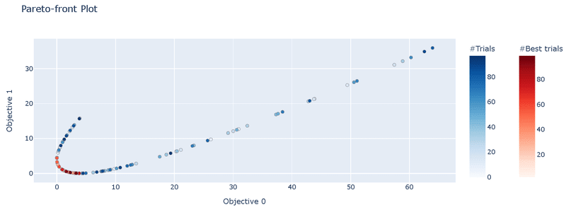
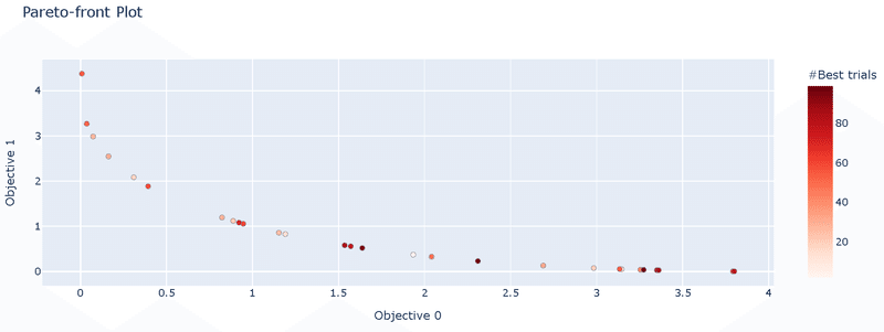
今回は$${f_1(x)}$$, $${f_2(x)}$$の最小化のためプロットは左下に寄る方がよいです。引数を指定することで非劣解のみを抽出できています。
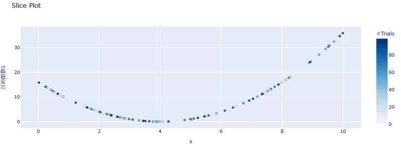
6-1-4.単目的最適化の可視化:plot_slice
多目的最適化の結果において、それぞれの目的関数の最適化の結果を表示するには"plot_slice"を使用します。
[API]
optuna.visualization.plot_slice(study, params=None, *,
target=None, target_name='Objective Value')最適化後のstudyとtargetを指定することで可視化可能です。
[IN]
optuna.visualization.plot_slice(study,
                                target=lambda t: t.values[0],
                                target_name='目的関数0').show()
optuna.visualization.plot_slice(study,
                                target=lambda t: t.values[1],
                                target_name='目的関数1').show()
[OUT]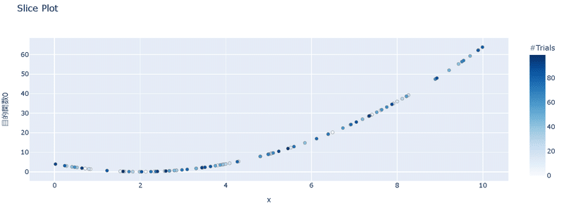
6-2.探索点の手動指定:Study.enqueue_trial
探索範囲をランダムに調整すると非常に時間がかかり計算資源も無駄になります。既によさそうなデータ(例:材料系の性能において論文データを参考など)がある場合、パラメータをその周辺で測定させると探索効率が上がることがあります。
Optunaでは"Study.enqueue_trial"で探索範囲の指定(事前知識)を追加することができ、サンプラーに探索のヒントを与えることが出来ます。
[API]
enqueue_trial(params, user_attrs=None, skip_if_exists=False)参考例として簡単にTitanicのデータを使用します。簡単な前処理として1.通常ないデータ(カラム)は削除、2.データが2種類:ラベルエンコーダー、3種以上:One-Hotで処理しました。
[IN]
from seaborn import load_dataset

titanic = load_dataset('titanic')
titanic = titanic.drop(columns=['alive', 'alone']) #Kaggleにないデータを削除
data_titanic, target_titanic = titanic.drop('survived', axis=1), titanic['survived']
# data_titanic.info() #データ型の確認

#ラベルエンコーディングとOne-Hotエンコーディング
for col in data_titanic.columns:
    # print(f'{col} : {data_titanic[col].nunique()}')
    #データ型がobjectかcategory,かつデータが2個ならラベルエンコーディング、3個以上ならOne-Hotエンコーディング
    if data_titanic[col].dtype.name in ['object', 'category'] and data_titanic[col].nunique() < 3:
        data_titanic[col] = data_titanic[col].astype('category').cat.codes #Category型に変換してからラベルエンコーディング
    elif data_titanic[col].dtype.name in ['object', 'category']:
        data_titanic = pd.get_dummies(data_titanic, columns=[col])

#NaNの処理
print(f'処理前データ数:{data_titanic.shape}')
data_titanic = data_titanic.fillna(data_titanic.mean())
print(f'処理後データ数:{data_titanic.shape}')
display(data_titanic)
# データセットの分割
X_train, X_test, y_train, y_test = train_test_split(data_titanic, target_titanic, test_size=0.2, random_state=0)
print(f'X_train:{len(X_train)} X_test:{len(X_test)}, y_train:{len(y_train)}, y_test:{len(y_test)}')
[OUT]
処理前データ数:(891, 26)
処理後データ数:(891, 26)
X_train:712 X_test:179, y_train:712, y_test:179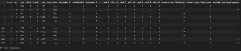
まずは事前知識は無しで通常通り実行します。Optunaで最適化することで手動で適当に設定したハイパーパラメータより性能(テストデータの精度)向上が確認されました。
[IN]
#手動で決定木を作成
tree_clf = DecisionTreeClassifier(random_state=0, max_depth=3, min_samples_leaf=2)
tree_clf.fit(X_train, y_train)  #学習 y_pred = tree_clf.predict(X_test) #予測
acc_train, acc_test = tree_clf.score(X_train, y_train), tree_clf.score(X_test, y_test)
print(f'正解率 訓練:{acc_train:.3f} テスト:{acc_test:.3f}')

#Optunaで決定木のパラメータ探索
def objective_tree(trial):
    max_depth = trial.suggest_int('max_depth', 1, 10)
    min_samples_leaf = trial.suggest_int('min_samples_leaf', 1, 10)

    tree_clf = DecisionTreeClassifier(random_state=0, max_depth=max_depth, min_samples_leaf=min_samples_leaf)
    tree_clf.fit(X_train, y_train)  #学習     y_pred = tree_clf.predict(X_test) #予測
    accuracy = tree_clf.score(X_test, y_test) #正解率
    return accuracy

study = optuna.create_study(direction='maximize')
study.optimize(objective_tree, n_trials=100)
print(f'最適化後 Params: {study.best_params}, Value: {study.best_value:.3f}')[OUT]
解率 訓練:0.834 テスト:0.816
[I 2023-04-15 20:22:25,390] A new study created in memory with name: no-name-24a7a0dc-d4af-44a1-9f70-bc422a295dad
[I 2023-04-15 20:22:25,399] Trial 0 finished with value: 0.8268156424581006 and parameters: {'max_depth': 5, 'min_samples_leaf': 7}. Best is trial 0 with value: 0.8268156424581006.
[I 2023-04-15 20:22:25,405] Trial 1 finished with value: 0.776536312849162 and parameters: {'max_depth': 1, 'min_samples_leaf': 2}. Best is trial 0 with value: 0.8268156424581006.
[I 2023-04-15 20:22:25,412] Trial 2 finished with value: 0.8212290502793296 and parameters: {'max_depth': 6, 'min_samples_leaf': 2}. Best is trial 0 with value: 0.8268156424581006.
・・・
[I 2023-04-15 20:22:26,628] Trial 97 finished with value: 0.8435754189944135 and parameters: {'max_depth': 10, 'min_samples_leaf': 5}. Best is trial 95 with value: 0.8435754189944135.
[I 2023-04-15 20:22:26,641] Trial 98 finished with value: 0.7877094972067039 and parameters: {'max_depth': 9, 'min_samples_leaf': 4}. Best is trial 95 with value: 0.8435754189944135.
[I 2023-04-15 20:22:26,654] Trial 99 finished with value: 0.7877094972067039 and parameters: {'max_depth': 9, 'min_samples_leaf': 4}. Best is trial 95 with value: 0.8435754189944135.
最適化後 Params: {'max_depth': 10, 'min_samples_leaf': 5}, Value: 0.844 次に事前知識を"Study.enqueue_trial"で追加してみます。"max_depth"は大きすぎると過学習しやすいですが少ないと精度が出ないため8程度、min_samples_leafは5くらいで情報を与えます。
Optunaの出力結果をみると"Study.enqueue_trial"で指定したパラメータ・値がTrial0, Trial1に反映されております。パラメータを指定することで探索空間のパラメータを指定できました。
[IN]
#Optunaで探索点の手動指定:Study.enqueue_trial

def objective_tree(trial):
    max_depth = trial.suggest_int('max_depth', 1, 10)
    min_samples_leaf = trial.suggest_int('min_samples_leaf', 1, 10)

    tree_clf = DecisionTreeClassifier(random_state=0, max_depth=max_depth, min_samples_leaf=min_samples_leaf)
    tree_clf.fit(X_train, y_train)  #学習     y_pred = tree_clf.predict(X_test) #予測
    accuracy = tree_clf.score(X_test, y_test) #正解率
    return accuracy

study2 = optuna.create_study(direction='maximize')

#探索点の手動指定:1回目のTrial
study2.enqueue_trial({'max_depth': 8, 'min_samples_leaf': 5})
#探索点の手動指定:2回目のTrial->max_depthだけ指定
study2.enqueue_trial({'max_depth': 9})

#最適化/結果の表示
study2.optimize(objective_tree, n_trials=100)
print(f'最適化後 Params: {study2.best_params}, Value: {study2.best_value:.3f}')
[OUT]
[I 2023-04-15 20:25:01,370] Trial 0 finished with value: 0.8324022346368715 and parameters: {'max_depth': 8, 'min_samples_leaf': 5}. Best is trial 0 with value: 0.8324022346368715.
[I 2023-04-15 20:25:01,377] Trial 1 finished with value: 0.8379888268156425 and parameters: {'max_depth': 9, 'min_samples_leaf': 9}. Best is trial 1 with value: 0.8379888268156425.
[I 2023-04-15 20:25:01,383] Trial 2 finished with value: 0.8268156424581006 and parameters: {'max_depth': 6, 'min_samples_leaf': 7}. Best is trial 1 with value: 0.8379888268156425.
[I 2023-04-15 20:25:01,390] Trial 3 finished with value: 0.8379888268156425 and parameters: {'max_depth': 10, 'min_samples_leaf': 9}. Best is trial 1 with value: 0.8379888268156425.
・・・
[I 2023-04-15 20:25:02,582] Trial 97 finished with value: 0.8379888268156425 and parameters: {'max_depth': 9, 'min_samples_leaf': 7}. Best is trial 1 with value: 0.8379888268156425.
[I 2023-04-15 20:25:02,595] Trial 98 finished with value: 0.8044692737430168 and parameters: {'max_depth': 9, 'min_samples_leaf': 5}. Best is trial 1 with value: 0.8379888268156425.
[I 2023-04-15 20:25:02,608] Trial 99 finished with value: 0.8268156424581006 and parameters: {'max_depth': 10, 'min_samples_leaf': 10}. Best is trial 1 with value: 0.8379888268156425.
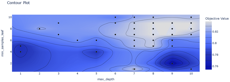
最適化後 Params: {'max_depth': 9, 'min_samples_leaf': 9}, Value: 0.838"Study.enqueue_trial"の有無における探索空間を等高線プロットで可視化すると、有りの方では指定した数値周辺の方が重点的に探索されています。
[IN]
optuna.visualization.plot_contour(study).show()
optuna.visualization.plot_contour(study2).show()

[OUT]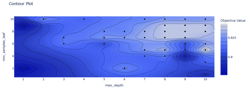
7.Webアプリ:Optuna Dashboard
Optunaの試行結果を確認できるWebアプリとしてOptuna Dashboardがあります。こちらはご紹介まで。
8.Optuna実践編
いくつかの事例を紹介しながら実践的な使い方を紹介します。
8-1.探索空間の可視化によるパラメータの影響確認
Optunaのslope_plot()を使用しながらハイパーパラメータの影響を可視化して、手動で探索空間を調整していきます。今回は”LightGBM”を使用して1.デフォルト、2.Optunaをシンプルに使用、3.探索空間を調整してOptunaを使用の3種で比較します。
まず初めにサンプルデータとしてTitanicを読み込みます。
[IN]
from seaborn import load_dataset

titanic = load_dataset('titanic')
titanic = titanic.drop(columns=['alive', 'alone']) #Kaggleにないデータを削除
data_titanic, target_titanic = titanic.drop('survived', axis=1), titanic['survived']
# data_titanic.info() #データ型の確認

#ラベルエンコーディングとOne-Hotエンコーディング
for col in data_titanic.columns:
    # print(f'{col} : {data_titanic[col].nunique()}')
    #データ型がobjectかcategory,かつデータが2個ならラベルエンコーディング、3個以上ならOne-Hotエンコーディング
    if data_titanic[col].dtype.name in ['object', 'category'] and data_titanic[col].nunique() < 3:
        data_titanic[col] = data_titanic[col].astype('category').cat.codes #Category型に変換してからラベルエンコーディング
    elif data_titanic[col].dtype.name in ['object', 'category']:
        data_titanic = pd.get_dummies(data_titanic, columns=[col])

#NaNの処理
print(f'処理前データ数:{data_titanic.shape}')
data_titanic = data_titanic.fillna(data_titanic.mean())
print(f'処理後データ数:{data_titanic.shape}')
display(data_titanic)
# データセットの分割
X_train, X_test, y_train, y_test = train_test_split(data_titanic, target_titanic, test_size=0.2, random_state=0)
print(f'X_train:{len(X_train)} X_test:{len(X_test)}, y_train:{len(y_train)}, y_test:{len(y_test)}')
[OUT]
処理前データ数:(891, 26)
処理後データ数:(891, 26)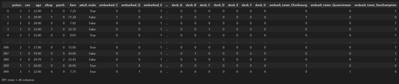
まずはLigthGBMを1.デフォルトで使用、2.Optunaをそのまま使用するパターンで処理します。それぞれ精度は84.4%, 86.6%でした。
[IN]
import lightgbm as lgb
from sklearn.model_selection import train_test_split
import sklearn.metrics as metrics

dtrain = lgb.Dataset(X_train, label=y_train)
print(dtrain, type(dtrain))

 #ハイパーパラメータ調整無し params = {"verbosity": -1}  #ログを出力しない gbm = lgb.train(params, dtrain)  #学習 y_pred_prob = gbm.predict(X_test) #予測
y_pred = np.rint(y_pred_prob) #四捨五入(0.5以上は1, 0.5未満は0)
accuracy = metrics.accuracy_score(y_test, y_pred) #正解率
print(f'精度(Default):{accuracy:.3f}')


 #Optunaでハイパーパラメータ調整 def objective(trial):
    dtrain = lgb.Dataset(X_train, label=y_train)  #データセットの作成     params = {
        "verbosity": -1,  #ログを出力しない         "max_bin": trial.suggest_int("max_bin", 10, 500),  #ヒストグラムのビンの数         "num_leaves": trial.suggest_int("num_leaves", 2, 500),  #木の葉の数         "min_data_in_leaf": trial.suggest_int("min_data_in_leaf", 2, 50),  #葉の最小データ数         "min_sum_hessian_in_leaf": trial.suggest_float("min_sum_hessian_in_leaf", 1e-8, 10.0, log=True),  #葉の最小ヘッシアン和         "bagging_fraction": trial.suggest_float("bagging_fraction", 0.1, 1.0),  #バギングの割合         "bagging_freq": trial.suggest_int("bagging_freq", 1, 100),  #バギングの頻度         "feature_fraction": trial.suggest_float("feature_fraction", 0.1, 1.0),  #特徴量の割合         "lambda_l1": trial.suggest_float("lambda_l1", 1e-8, 10.0, log=True),  #L1正則化の強さ         "lambda_l2": trial.suggest_float("lambda_l2", 1e-8, 10.0, log=True),  #L2正則化の強さ         "min_gain_to_split": trial.suggest_float("min_gain_to_split", 0, 10),  #分割に必要な最小損失         "max_depth": trial.suggest_int("max_depth", 2, 100),  #木の深さ         "extra_trees": trial.suggest_categorical("extra_trees", [True, False]),  #ExtraTreesを使用するか         "path_smooth": trial.suggest_int("path_smooth", 0, 10),  #パススムージングの強さ     }
    gbm = lgb.train(params, dtrain)  #学習     y_preds_prob = gbm.predict(X_test) #予測
    y_preds = np.rint(y_preds_prob) #四捨五入(0.5以上は1, 0.5未満は0)
    accuracy = metrics.accuracy_score(y_test, y_preds) #正解率

    return accuracy

study = optuna.create_study(
    study_name='visualize_hyperparameter_LightGBM',
    storage='sqlite:///optuna.db',
    direction='maximize')

study.optimize(objective, n_trials=100)

trial = study.best_trial
print(f'Accuracy: {trial.value}')
for key, value in trial.params.items():
    print(f'{key}: {value}')
[OUT]
精度(Default):0.844
Accuracy: 0.8659217877094972
bagging_fraction: 0.9208588588605883
bagging_freq: 11
extra_trees: False
feature_fraction: 0.718069205176339
lambda_l1: 7.245698690575839e-08
lambda_l2: 0.004018763924208708
max_bin: 447
max_depth: 75
min_data_in_leaf: 11
min_gain_to_split: 0.02511794186773987
min_sum_hessian_in_leaf: 0.02482164452037786
num_leaves: 436
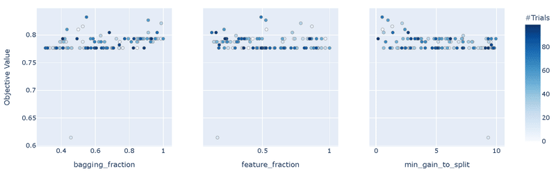
path_smooth: 4次に探索空間を可視化して最適な範囲を調整します。今回の目的は探索空間を分析のためサンプラーはRandomSamplerを使用します。流れとしては下記となります。
"RandomSampler"によりランダムにパラメータを選定して性能評価
"plot_param_importances"でパラメータの重要度を可視化
重要度が高いパラメータを"plot_slice()"で可視化して、性能とパラメータの相関関係を確認(※因果関係ではないことに注意)
確認した相関関係からパラメータの探索範囲を調整(性能が低くなる範囲は探索しないように設定)
1~4を繰り返し
それでは実際にやってみます。変更箇所は"optuna.create_study"のサンプラーに"RandomSampler"を追加しました。結果として下記が確認できます。
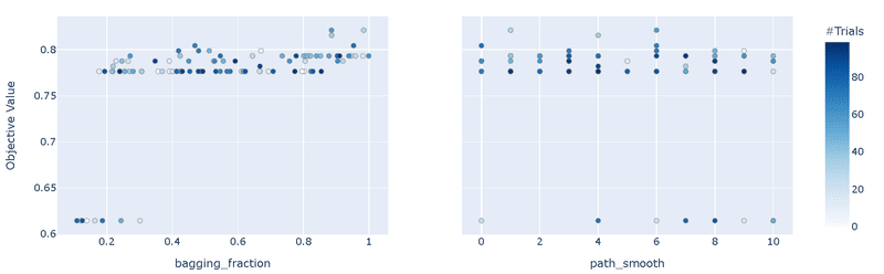
"RandomSampler"のため精度は最適化(TPESampler)より悪い
重要度として"bagging_fraction"の影響が圧倒的に大きい
bagging_fractionのplot_slice()より、値は0.3以上の方がよさそう
[IN]
 #Optunaでハイパーパラメータ調整 def objective(trial):
    dtrain = lgb.Dataset(X_train, label=y_train)  #データセットの作成     params = {
        "verbosity": -1,  #ログを出力しない
        "max_bin": trial.suggest_int("max_bin", 10, 500),  #ヒストグラムのビンの数         "num_leaves": trial.suggest_int("num_leaves", 2, 500),  #木の葉の数         "min_data_in_leaf": trial.suggest_int("min_data_in_leaf", 2, 50),  #葉の最小データ数         "min_sum_hessian_in_leaf": trial.suggest_float("min_sum_hessian_in_leaf", 1e-8, 10.0, log=True),  #葉の最小ヘッシアン和         "bagging_fraction": trial.suggest_float("bagging_fraction", 0.1, 1.0),  #バギングの割合         "bagging_freq": trial.suggest_int("bagging_freq", 1, 100),  #バギングの頻度         "feature_fraction": trial.suggest_float("feature_fraction", 0.1, 1.0),  #特徴量の割合         "lambda_l1": trial.suggest_float("lambda_l1", 1e-8, 10.0, log=True),  #L1正則化の強さ         "lambda_l2": trial.suggest_float("lambda_l2", 1e-8, 10.0, log=True),  #L2正則化の強さ         "min_gain_to_split": trial.suggest_float("min_gain_to_split", 0, 10),  #分割に必要な最小損失         "max_depth": trial.suggest_int("max_depth", 2, 100),  #木の深さ         "extra_trees": trial.suggest_categorical("extra_trees", [True, False]),  #ExtraTreesを使用するか         "path_smooth": trial.suggest_int("path_smooth", 0, 10),  #パススムージングの強さ     }
    gbm = lgb.train(params, dtrain)  #学習     y_preds_prob = gbm.predict(X_test) #予測
    y_preds = np.rint(y_preds_prob) #四捨五入(0.5以上は1, 0.5未満は0)
    accuracy = metrics.accuracy_score(y_test, y_preds) #正解率

    return accuracy

study = optuna.create_study(
    study_name='viz_hyperparameter_LightGBM',
    storage='sqlite:///optuna.db',
    direction='maximize',
    sampler=optuna.samplers.RandomSampler(seed=1234))

study.optimize(objective, n_trials=100)

trial = study.best_trial
print(f'Accuracy: {trial.value}')
for key, value in trial.params.items():
    print(f'{key}: {value}')


optuna.visualization.plot_param_importances(study).show()
optuna.visualization.plot_slice(study, params=['bagging_fraction', 'path_smooth']).show()
[OUT]
Accuracy: 0.8212290502793296
bagging_fraction: 0.9834887945246333
bagging_freq: 70
extra_trees: False
feature_fraction: 0.7857765037325378
lambda_l1: 6.712474443664293e-05
lambda_l2: 1.7784472805864132e-07
max_bin: 342
max_depth: 77
min_data_in_leaf: 9
min_gain_to_split: 2.161863031600805
min_sum_hessian_in_leaf: 0.007014871557519257
num_leaves: 72
path_smooth: 1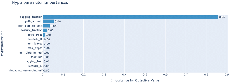
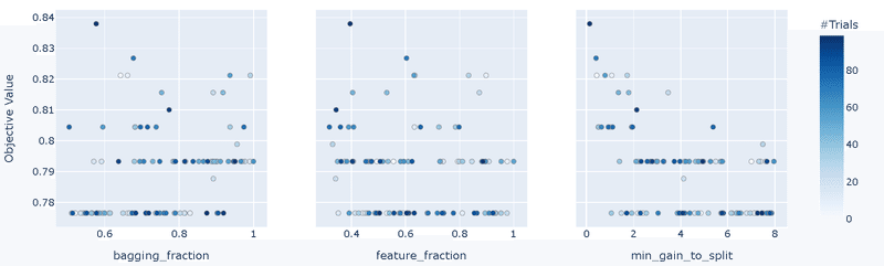
Paramsの"bagging_fraction"の下限を0.3に変更して再度実行します。結果は下記の通りです。
前回結果より精度が改善された(0.82->0.83)
重要度として3つのパラメータの影響が大きい
傾向が判断しにくいが"min_gain_to_split"は低めの方がよさそう
[IN]
 #Optunaでハイパーパラメータ調整 def objective(trial):
    dtrain = lgb.Dataset(X_train, label=y_train)  #データセットの作成     params = {
        "verbosity": -1,  #ログを出力しない
        "max_bin": trial.suggest_int("max_bin", 10, 500),  #ヒストグラムのビンの数         "num_leaves": trial.suggest_int("num_leaves", 2, 500),  #木の葉の数         "min_data_in_leaf": trial.suggest_int("min_data_in_leaf", 2, 50),  #葉の最小データ数         "min_sum_hessian_in_leaf": trial.suggest_float("min_sum_hessian_in_leaf", 1e-8, 10.0, log=True),  #葉の最小ヘッシアン和         "bagging_fraction": trial.suggest_float("bagging_fraction", 0.3, 1.0),  #バギングの割合         "bagging_freq": trial.suggest_int("bagging_freq", 1, 100),  #バギングの頻度         "feature_fraction": trial.suggest_float("feature_fraction", 0.1, 1.0),  #特徴量の割合         "lambda_l1": trial.suggest_float("lambda_l1", 1e-8, 10.0, log=True),  #L1正則化の強さ         "lambda_l2": trial.suggest_float("lambda_l2", 1e-8, 10.0, log=True),  #L2正則化の強さ         "min_gain_to_split": trial.suggest_float("min_gain_to_split", 0, 10),  #分割に必要な最小損失         "max_depth": trial.suggest_int("max_depth", 2, 100),  #木の深さ         "extra_trees": trial.suggest_categorical("extra_trees", [True, False]),  #ExtraTreesを使用するか         "path_smooth": trial.suggest_int("path_smooth", 0, 10),  #パススムージングの強さ     }
    gbm = lgb.train(params, dtrain)  #学習     y_preds_prob = gbm.predict(X_test) #予測
    y_preds = np.rint(y_preds_prob) #四捨五入(0.5以上は1, 0.5未満は0)
    accuracy = metrics.accuracy_score(y_test, y_preds) #正解率

    return accuracy

study2 = optuna.create_study(
    study_name='viz_hyperparameter2_LightGBM',
    storage='sqlite:///optuna.db',
    direction='maximize',
    sampler=optuna.samplers.RandomSampler(seed=1234))

study2.optimize(objective, n_trials=100)

trial = study2.best_trial
print(f'Accuracy: {trial.value}')
for key, value in trial.params.items():
    print(f'{key}: {value}')


optuna.visualization.plot_param_importances(study2).show()
optuna.visualization.plot_slice(study2, params=['min_gain_to_split', 'bagging_fraction', 'feature_fraction']).show()
[OUT]
Accuracy: 0.8324022346368715
bagging_fraction: 0.547969014034902
bagging_freq: 92
extra_trees: False
feature_fraction: 0.49016882713895227
lambda_l1: 4.0240463730214977e-07
lambda_l2: 0.05881122718152152
max_bin: 241
max_depth: 10
min_data_in_leaf: 12
min_gain_to_split: 0.5047056570277519
min_sum_hessian_in_leaf: 3.9614702773504775e-07
num_leaves: 102
path_smooth: 6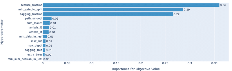
Paramsの['min_gain_to_split', 'bagging_fraction', 'feature_fraction']を調整して再度実行します。結果は下記の通りです。
前回結果より精度が改善された(0.832->0.838)
重要度が大きいパラメータは前回と同じ
"min_gain_to_split"は低めの方がよさそう
[IN]
 #Optunaでハイパーパラメータ調整 def objective(trial):
    dtrain = lgb.Dataset(X_train, label=y_train)  #データセットの作成     params = {
        "verbosity": -1,  #ログを出力しない
        "max_bin": trial.suggest_int("max_bin", 10, 500),  #ヒストグラムのビンの数         "num_leaves": trial.suggest_int("num_leaves", 2, 500),  #木の葉の数         "min_data_in_leaf": trial.suggest_int("min_data_in_leaf", 2, 50),  #葉の最小データ数         "min_sum_hessian_in_leaf": trial.suggest_float("min_sum_hessian_in_leaf", 1e-8, 10.0, log=True),  #葉の最小ヘッシアン和         "bagging_fraction": trial.suggest_float("bagging_fraction", 0.5, 1.0),  #バギングの割合         "bagging_freq": trial.suggest_int("bagging_freq", 1, 100),  #バギングの頻度         "feature_fraction": trial.suggest_float("feature_fraction", 0.3, 1.0),  #特徴量の割合         "lambda_l1": trial.suggest_float("lambda_l1", 1e-8, 10.0, log=True),  #L1正則化の強さ         "lambda_l2": trial.suggest_float("lambda_l2", 1e-8, 10.0, log=True),  #L2正則化の強さ         "min_gain_to_split": trial.suggest_float("min_gain_to_split", 0, 8),  #分割に必要な最小損失         "max_depth": trial.suggest_int("max_depth", 2, 100),  #木の深さ         "extra_trees": trial.suggest_categorical("extra_trees", [True, False]),  #ExtraTreesを使用するか         "path_smooth": trial.suggest_int("path_smooth", 0, 10),  #パススムージングの強さ     }
    gbm = lgb.train(params, dtrain)  #学習     y_preds_prob = gbm.predict(X_test) #予測
    y_preds = np.rint(y_preds_prob) #四捨五入(0.5以上は1, 0.5未満は0)
    accuracy = metrics.accuracy_score(y_test, y_preds) #正解率

    return accuracy

study3 = optuna.create_study(
    study_name='viz_hyperparameter3_LightGBM',
    storage='sqlite:///optuna.db',
    direction='maximize',
    sampler=optuna.samplers.RandomSampler(seed=1234))

study3.optimize(objective, n_trials=100)

trial = study3.best_trial
print(f'Accuracy: {trial.value}')
for key, value in trial.params.items():
    print(f'{key}: {value}')


optuna.visualization.plot_param_importances(study3).show()
optuna.visualization.plot_slice(study3, params=['min_gain_to_split', 'bagging_fraction', 'feature_fraction']).show()
[OUT]
Accuracy: 0.8379888268156425
bagging_fraction: 0.5773029175673157
bagging_freq: 72
extra_trees: False
feature_fraction: 0.3947848313836965
lambda_l1: 1.0987988535264347e-08
lambda_l2: 0.0006880905358918668
max_bin: 318
max_depth: 55
min_data_in_leaf: 5
min_gain_to_split: 0.13274241507422513
min_sum_hessian_in_leaf: 0.0008987280305939641
num_leaves: 454
path_smooth: 9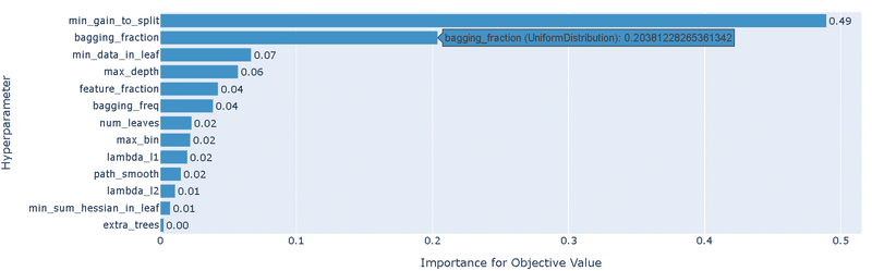
Paramsの"min_gain_to_split"の上限を4に変更し、サンプラーをデフォルト(TPESampler)に戻して実行します。探索空間をよさそうな範囲に狭めているためうまくいけばより精度が上がります。結果は下記の通りです。
精度は86.6%のため今回はデフォルトとの差は確認されなかった。(公式図書の事例でも84.7%->86.7%であり飛びぬけた改善は期待できない)
デフォルトの場合より最適解に到達するTrial回数が短い。つまりより良い探索空間を調査できている。
[IN]
 #Optunaでハイパーパラメータ調整 def objective(trial):
    dtrain = lgb.Dataset(X_train, label=y_train)  #データセットの作成     params = {
        "verbosity": -1,  #ログを出力しない
        "max_bin": trial.suggest_int("max_bin", 10, 500),  #ヒストグラムのビンの数         "num_leaves": trial.suggest_int("num_leaves", 2, 500),  #木の葉の数         "min_data_in_leaf": trial.suggest_int("min_data_in_leaf", 2, 50),  #葉の最小データ数         "min_sum_hessian_in_leaf": trial.suggest_float("min_sum_hessian_in_leaf", 1e-8, 10.0, log=True),  #葉の最小ヘッシアン和         "bagging_fraction": trial.suggest_float("bagging_fraction", 0.5, 1.0),  #バギングの割合         "bagging_freq": trial.suggest_int("bagging_freq", 1, 100),  #バギングの頻度         "feature_fraction": trial.suggest_float("feature_fraction", 0.3, 0.9),  #特徴量の割合         "lambda_l1": trial.suggest_float("lambda_l1", 1e-8, 10.0, log=True),  #L1正則化の強さ         "lambda_l2": trial.suggest_float("lambda_l2", 1e-8, 10.0, log=True),  #L2正則化の強さ         "min_gain_to_split": trial.suggest_float("min_gain_to_split", 0, 4),  #分割に必要な最小損失         "max_depth": trial.suggest_int("max_depth", 2, 100),  #木の深さ         "extra_trees": trial.suggest_categorical("extra_trees", [True, False]),  #ExtraTreesを使用するか         "path_smooth": trial.suggest_int("path_smooth", 0, 10),  #パススムージングの強さ     }
    gbm = lgb.train(params, dtrain)  #学習     y_preds_prob = gbm.predict(X_test) #予測
    y_preds = np.rint(y_preds_prob) #四捨五入(0.5以上は1, 0.5未満は0)
    accuracy = metrics.accuracy_score(y_test, y_preds) #正解率

    return accuracy

study_final = optuna.create_study(
    study_name='visualize_hyperparameter_LightGBM_final',
    storage='sqlite:///optuna.db',
    direction='maximize')

study_final.optimize(objective, n_trials=100)

trial = study_final.best_trial
print(f'Accuracy: {trial.value}')
for key, value in trial.params.items():
    print(f'{key}: {value}')

optuna.visualization.plot_optimization_history(study1st).show()
optuna.visualization.plot_optimization_history(study_final).show()
[OUT]
Accuracy: 0.8659217877094972
bagging_fraction: 0.9130513652401059
bagging_freq: 83
extra_trees: False
feature_fraction: 0.612264513790025
lambda_l1: 2.992711564682563e-08
lambda_l2: 2.2771877506914086e-05
max_bin: 269
max_depth: 58
min_data_in_leaf: 34
min_gain_to_split: 0.0017115052641551894
min_sum_hessian_in_leaf: 2.0572813275603016e-08
num_leaves: 286
path_smooth: 0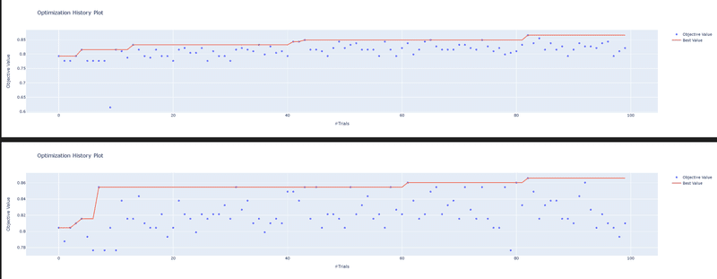
8-2.NNモデルの最適化
深層学習の全結合モデル(MLP)は表現力を高くできる反面、下記のように多くのハイパーパラメータを調整する必要があります。
Layer(層)数
Layerのノード数
活性化関数
最適化関数
ドロップアウト率/BatchNormalization
学習率
Early Stoppingの有無
依然の記事では感覚(入力次元情報を削減しないように大きめのノード+層)で設計しましたが、今回はOptunaで実験してみます。
今回もTitanicのデータを使用するため簡単な前処理を実施しました。前節と異なり(木構造モデルでは問題ないですが)、全結合モデルは標準化/正規化が必須のためsklearnの"StandardScaler"で標準化しました。また後でPytorchのTensorに変換しやすいようにNumpy型でデータを準備します。
[IN]
import torch
import torch.nn as nn
import torch.nn.functional as F
import torch.optim as optim
from torchinfo import summary
from tqdm import tqdm
import numpy as np
import pandas as pd
import matplotlib.pyplot as plt
import seaborn as sns

from seaborn import load_dataset
from sklearn.preprocessing import StandardScaler
from sklearn.model_selection import train_test_split
from sklearn.metrics import accuracy_score

titanic = load_dataset('titanic')
titanic = titanic.drop(columns=['alive', 'alone']) #Kaggleにないデータを削除
data_titanic, target_titanic = titanic.drop('survived', axis=1), titanic['survived']
# data_titanic.info() #データ型の確認

#ラベルエンコーディングとOne-Hotエンコーディング
for col in data_titanic.columns:
    # print(f'{col} : {data_titanic[col].nunique()}')
    #データ型がobjectかcategory,かつデータが2個ならラベルエンコーディング、3個以上ならOne-Hotエンコーディング
    if data_titanic[col].dtype.name in ['object', 'category'] and data_titanic[col].nunique() < 3:
        data_titanic[col] = data_titanic[col].astype('category').cat.codes #Category型に変換してからラベルエンコーディング
    elif data_titanic[col].dtype.name in ['object', 'category']:
        data_titanic = pd.get_dummies(data_titanic, columns=[col])

#NaNの処理
print(f'処理前データ数:{data_titanic.shape}')
data_titanic = data_titanic.fillna(data_titanic.mean())
print(f'処理後データ数:{data_titanic.shape}')
# print(data_titanic.isnull().sum())  #NaNの確認
display(data_titanic)
# データセットの分割
X_train, X_test, y_train, y_test = train_test_split(data_titanic, target_titanic, test_size=0.2, random_state=0)
print(f'X_train:{type(X_train)} X_test:{type(X_test)}, y_train:{type(y_train)}, y_test:{type(y_test)}')

#標準化:NN使用のため, また説明変数に合わせてテストデータもNumpy配列に変換
scaler = StandardScaler()
X_train = scaler.fit_transform(X_train)
X_test = scaler.transform(X_test)
y_train, y_test = y_train.values, y_test.values
print(f'X_train:{type(X_train)} X_test:{type(X_test)}, y_train:{type(y_train)}, y_test:{type(y_test)}')
[OUT]
処理前データ数:(891, 26)
処理後データ数:(891, 26)
X_train:<class 'pandas.core.frame.DataFrame'> X_test:<class 'pandas.core.frame.DataFrame'>, y_train:<class 'pandas.core.series.Series'>, y_test:<class 'pandas.core.series.Series'>
X_train:<class 'numpy.ndarray'> X_test:<class 'numpy.ndarray'>, y_train:<class 'numpy.ndarray'>, y_test:<class 'numpy.ndarray'>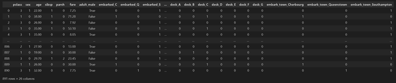
まず初めに直感で全結合モデルモデルを作成して性能を確認しました。精度は80.4%とまずまずの結果です。
[IN]
import optuna
import torch
import torch.nn as nn
import torch.optim as optim
from torch.utils.data import DataLoader, TensorDataset
from typing import Tuple
from tqdm import tqdm

class Net(nn.Module):
    def __init__(self, in_size, out_size):
        super(Net, self).__init__()
        self.fc1 = nn.Linear(in_size, 128)
        self.fc2 = nn.Linear(128, 64)
        self.fc3 = nn.Linear(64, 32)
        self.fc4 = nn.Linear(32, out_size)
        self.relu = nn.ReLU()
        self.softmax = nn.Softmax(dim=1)

    def forward(self, x):
        x = self.relu(self.fc1(x))
        x = self.relu(self.fc2(x))
        x = self.relu(self.fc3(x))
        x = self.softmax(self.fc4(x)) #ソフトマックス関数 ->2値を確率で出力
        return x

# データセットの作成
X_train_tensor = torch.tensor(X_train, dtype=torch.float32)
X_test_tensor = torch.tensor(X_test, dtype=torch.float32)
y_train_tensor = torch.tensor(y_train, dtype=torch.long)
y_test_tensor = torch.tensor(y_test, dtype=torch.long)

# ハイパーパラメータの設定
device = 'cuda' if torch.cuda.is_available() else 'cpu'
epochs = 100
lr = 0.01 #学習率
def logging_epoch(logs, epoch, loss, acc): #学習結果を辞書に格納する関数
    logs['epoch'].append(epoch) #学習回数を格納
    logs['loss'].append(loss) #損失関数を格納
    logs['accuracy'].append(acc) #正解率を格納

logs = {'train':{'epoch':[], 'loss':[], 'accuracy':[]},
        'val':{'epoch':[], 'loss':[], 'accuracy':[]},
        'test':{'epoch':[], 'loss':[], 'accuracy':[]}} #学習結果を格納する辞書

# モデルの定義
net = Net(in_size=X_train_tensor.shape[1], out_size=2)
optimizer = optim.Adam(net.parameters(), lr=lr)
critertion = nn.CrossEntropyLoss() #交差エントロピー誤差関数
 #GPU使用
X_train_tensor, X_test_tensor, y_train_tensor, y_test_tensor = X_train_tensor.to(device), X_test_tensor.to(device), y_train_tensor.to(device), y_test_tensor.to(device)
net = net.to(device)

for epoch in tqdm(range(epochs)):
    for phase in ['train', 'val']:
        if phase == 'train':
            net.train()
        else:
            net.eval()

        if phase == 'train':
            optimizer.zero_grad() #勾配の初期化
            output = net(X_train_tensor)
            loss = critertion(output, y_train_tensor)
            loss.backward() #勾配の計算
            optimizer.step()

        if epoch % 10 == 0:
            if phase == 'train':
                acc = (output.argmax(dim=1) == y_train_tensor).float().mean()
                logging_epoch(logs['train'], epoch, loss.item(), acc.item())

            elif phase == 'val':
                y_pred_test = net(X_test_tensor)
                loss_test = critertion(y_pred_test, y_test_tensor)
                acc = (y_pred_test.argmax(dim=1) == y_test_tensor).float().mean()
                logging_epoch(logs['test'], epoch, loss_test.item(), acc.item())


summary_model = summary(net, (1, X_train_tensor.shape[1])) # モデルの概要を表示
print(summary_model)
 #学習時・検証時の損失の推移を可視化
fig, ax = plt.subplots(1, 1, figsize=(8, 6))
ax.plot(logs['train']['epoch'], logs['train']['accuracy'],
        label='train', color='blue', linewidth=1, alpha=0.5, linestyle='--')
ax.plot(logs['test']['epoch'], logs['test']['accuracy'],
        label='test', color='red', linewidth=1, alpha=0.5, linestyle='-')
plt.grid(), plt.legend()

y_pred_test = net(X_test_tensor)
accuracy_score(y_test_tensor.cpu().detach().numpy(), y_pred_test.cpu().detach().numpy().argmax(axis=1))[OUT]
==========================================================================================
Layer (type:depth-idx) Output Shape Param #
==========================================================================================
Net -- --
├─Linear: 1-1 [1, 128] 3,456
├─ReLU: 1-2 [1, 128] --
├─Linear: 1-3 [1, 64] 8,256
├─ReLU: 1-4 [1, 64] --
├─Linear: 1-5 [1, 32] 2,080
├─ReLU: 1-6 [1, 32] --
├─Linear: 1-7 [1, 2] 66
├─Softmax: 1-8 [1, 2] --
==========================================================================================
Total params: 13,858
Trainable params: 13,858
Non-trainable params: 0
Total mult-adds (M): 0.01
==========================================================================================
Input size (MB): 0.00
Forward/backward pass size (MB): 0.00
Params size (MB): 0.06
Estimated Total Size (MB): 0.06
==========================================================================================
0.8044692737430168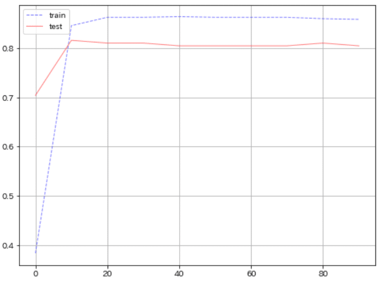
次にOptunaでハイパーパラメータを最適化します。学習率は固定値、Early Stoppingは無し(代わりに参考用としてOptunaの枝刈り(TrialPruned()を追加)で実行しました。
Layer(層)数:1~3層
Layerのノード数:4~128ノード
活性化関数:ReLUまたはTanh
最適化関数:SGDまたはAdam
ドロップアウト率:0~0.5
結果として精度が80.4->83.2%に向上しました。なお乱数固定されていないため毎回結果は変わります(10回くらいやった結果も載せました)。
[IN]
# 必要なライブラリをインポート
import optuna
import torch
import torch.nn as nn
import torch.optim as optim
from torch.utils.data import DataLoader, TensorDataset
from typing import Tuple

# PyTorchのニューラルネットワークモデルを定義
class Net(nn.Module):
    def __init__(self, input_size: int, output_size: int, hidden_layers: Tuple[int], activation: nn.Module, dropout_rate: float):
        super(Net, self).__init__()
        layers = [] #NN層を格納するリスト
        in_features = input_size # 入力層のユニット数

        for out_features in hidden_layers:
            layers.append(nn.Linear(in_features, out_features)) #中間層 (Affine Layer)
            layers.append(activation) # 活性化関数
            layers.append(nn.Dropout(dropout_rate))  # ドロップアウト層
            in_features = out_features # 使用したLayerの次の前のLayerとする

        layers.append(nn.Linear(in_features, output_size))
        self.model = nn.Sequential(*layers)

    def forward(self, x: torch.Tensor) -> torch.Tensor:
        return self.model(x)

# Optunaを使ってハイパーパラメータを最適化する関数を定義
def objective(trial: optuna.Trial) -> float:
    # ハイパーパラメータの探索範囲を定義
    n_layers = trial.suggest_int("n_layers", 1, 3)
    hidden_units = [trial.suggest_int(f"n_units_{i}", 4, 128) for i in range(n_layers)]
    activation_name = trial.suggest_categorical("activation", ["ReLU", "Tanh"])
    optimizer_name = trial.suggest_categorical("optimizer", ["SGD", "Adam"])
    dropout_rate = trial.suggest_float("dropout_rate", 0.0, 0.5)  # ドロップアウト率の探索

    # 活性化関数とオプティマイザの選択
    activation = nn.ReLU() if activation_name == "ReLU" else nn.Tanh()
    optimizer_class = optim.SGD if optimizer_name == "SGD" else optim.Adam

    # モデルを構築
    input_size = X_train.shape[1] # 入力層のユニット数(説明変数の次元数)
    output_size = 2 #損失関数で多クラス用のCrossEntropyLossを使用するため 、出力層のユニット数は2
    model = Net(input_size, output_size, hidden_units, activation, dropout_rate)

    # オプティマイザを設定
    optimizer = optimizer_class(model.parameters(), lr=0.01)

    # 訓練データをDataLoaderにロード
    X_train_tensor = torch.tensor(X_train.astype(np.float32), dtype=torch.float)
    y_train_tensor = torch.tensor(y_train, dtype=torch.long)
    train_dataset = TensorDataset(X_train_tensor, y_train_tensor)
    train_loader = DataLoader(train_dataset, batch_size=32)

    # モデルの訓練
    for epoch in range(10):
        for batch in train_loader:
            optimizer.zero_grad() # 勾配の初期化
            x, y = batch
            y_pred = model(x) #推論
            loss = nn.CrossEntropyLoss()(y_pred, y) #損失関数 ※多クラス用
            loss.backward() #勾配の計算
            optimizer.step() #パラメータの更新

        # Optunaの枝刈り機能を利用して、訓練途中で性能が低いモデルを打ち切り
        intermediate_value = loss.item()
        trial.report(intermediate_value, epoch)
        if trial.should_prune():
            raise optuna.exceptions.TrialPruned() #枝刈り (Early Stopping)

    # モデルの評価
    X_test_tensor = torch.tensor(X_test.astype(np.float32), dtype=torch.float) #DataFrameにintとfloatが混在しているため 、float32に変換
    y_test_tensor = torch.tensor(y_test, dtype=torch.long)
    test_dataset = TensorDataset(X_test_tensor, y_test_tensor)
    test_loader = DataLoader(test_dataset, batch_size=32)
    correct = 0
    total = 0
    with torch.no_grad():
        for batch in test_loader:
            x, y = batch
            y_pred = model(x)
            _, predicted = torch.max(y_pred.data, 1)
            total += y.size(0)
            correct += (predicted == y).sum().item()

    accuracy = correct / total
    return accuracy

# Optunaを使ってハイパーパラメータチューニングを実行
study = optuna.create_study(direction="maximize", pruner=optuna.pruners.MedianPruner())
study.optimize(objective, n_trials=100)

# 最適なハイパーパラメータを表示
print("Best trial:")
trial = study.best_trial
print(f"  Value: {trial.value}")
print("  Params: ")
for key, value in trial.params.items():
    print(f"{key}: {value}")
[OUT]
Best trial:
Value: 0.8324022346368715
Params:
n_layers: 3
n_units_0: 81
n_units_1: 24
n_units_2: 6
activation: ReLU
optimizer: Adam
dropout_rate: 0.4567835224784788[OUT]※たまたまでたMAX
Best trial:
Value: 0.8435754189944135
Params:
n_layers: 2
n_units_0: 31
n_units_1: 108
activation: ReLU
optimizer: SGD
dropout_rate: 0.01780306168515259.補足 Optunaのアルゴリズム:Sampler
Optunaでは多目的最適化において探索空間内の1点を選択(探索点選択)アルゴリズムをSamplerというクラスで実装されています。アルゴリズムには特徴がありトライアル数が少ないと精度が出ないもの(進化計算(NSGAなど)や動作速度が速いものなどがあるため、用途に応じて選定する必要があります。
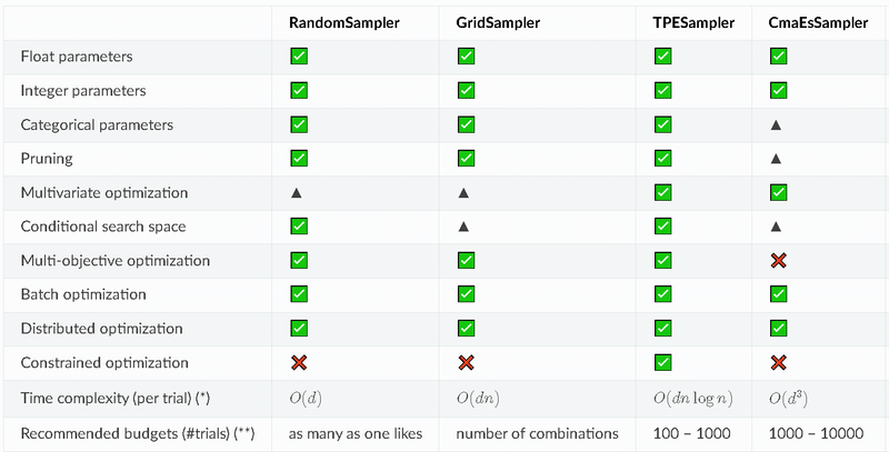
BaseSampler: すべてのサンプラーの基本となるクラス。他のサンプラーはこのクラスを継承して実装されます。
GridSampler: グリッドサーチを使用するサンプラー。事前に定義されたハイパーパラメータの組み合わせを試す。
RandomSampler: ランダムサンプリングを使用するサンプラー。ハイパーパラメータの値を無作為に選択する。
TPESampler: TPE (Tree-structured Parzen Estimator) アルゴリズムを使用するサンプラー。過去の試行結果をもとに、次に試すべきハイパーパラメータの値を決定する。
CmaEsSampler: CMA-ES (Covariance Matrix Adaptation Evolution Strategy) アルゴリズムを使用するサンプラー。連続値のハイパーパラメータに対して最適化を行う。
PartialFixedSampler: 一部のハイパーパラメータが固定されたサンプラー。特定のハイパーパラメータを固定し、他のハイパーパラメータの最適化を行う。
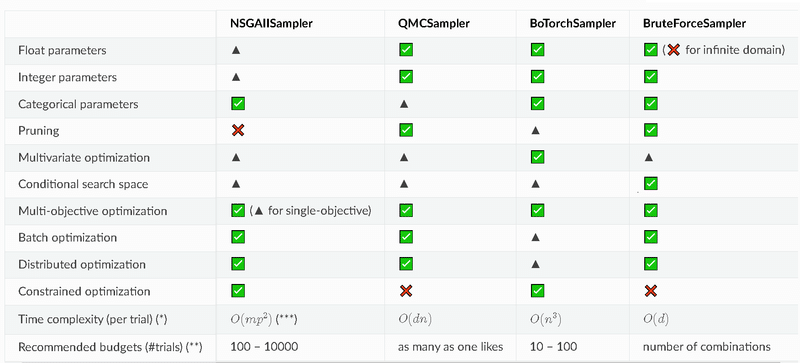
NSGAIISampler: NSGA-II (Non-dominated Sorting Genetic Algorithm II) アルゴリズムを使用する多目的最適化サンプラー。複数の目的関数を最適化する問題に対応。
MOTPESampler: MOTPE (Multi-Objective Tree-structured Parzen Estimator) アルゴリズムを使用する多目的最適化サンプラー。複数の目的関数を最適化する問題に対応。
QMCSampler: 低離散度列を生成するクォーシモンテカルロ (Quasi Monte Carlo) サンプラー。ランダムサンプリングよりも効率的に探索空間をカバーする。
BruteForceSampler: ブルートフォースを使用するサンプラー。探索空間のすべてのハイパーパラメータの組み合わせを試す。
IntersectionSearchSpace: 研究の交差探索空間を計算
9-1.TPESampler:ベイズ最適化(単目的最適化)
Optunaの単目的最適化のデフォルトはTPE(Tree-structured Parzen Estimator)です。"Tree-structured"はforループやif文を含むことにより探索空間中のパラメータの関係が木構造になっている場合にも対応できることを表しています。
なお多目的最適化のデフォルトはNSGAIISampler(アルゴリズム:進化計算)です。動作速度が速く制約付き最適にも対応している特徴があります。
9-2.BoTorchSampler:ベイズ最適化
Optunaに実装されているBoTorchSamplerはMeta社が開発するベイズ最適化ライブラリBoTorchをOptuna側でカスタムしたものになります。
参考資料
あとがき
今度コンペで使用してみたい!。ただ、結構多くのコンペではハイパラ調整より特徴量の作りこみが甘いことがあるし、ハイパラ最適化の効果はよくて数%くらいなのは肝に銘じておきたい。
この記事が気に入ったらサポートをしてみませんか?