
Pythonライブラリ:scikit-learn (前処理・Score確認編)

概要
機械学習用パッケージのscikit-learn(sklearn)を紹介します。sklearnは様々な機械学習を簡単に実装できます。本記事では機械学習を実施するためのデータの前処理や学習方法をメインに紹介します。
1.基礎知識
1-1.AI・ML・DLの違い
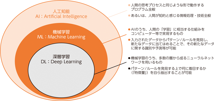
前提知識として下図より、AI>機械学習>深層学習の関係にあります(第1部 特集 進化するデジタル経済とその先にあるSociety 5.0 参照)。
また機械学習は3分類に分けられます(種類としては「自己教師あり学習」もあります)。

1-2.機械学習(AIモデル)の訓練の流れ
機械学習でのモデル訓練の大まかな流れは下記の通りです。
【訓練の流れ】
1.データセットの準備
2.AIモデルの選定
3.目的関数(損失関数)の選定
4.最適化手法の選定
5.モデルの学習
1-3.データセットの分割:学習・検証・テスト用
機械学習では学習結果の精度は高いが実際のデータでは精度が低くなることがあり過学習と呼ばれます。その防止として、学習時に学習・検証用データセットで学習して、実際の精度確認はテスト用データで実施します。
2.サンプルデータセット
2-1.sklearn内のデータの取得:load_x()
scikit-learnはload_xxx()でサンプルデータを取得できます。通常業務では自分のデータを使用しますが今回は説明用としてサンプルデータを使用します。
【確認用コード】
[In]
from sklearn import datasets
iris = datasets.load_iris() #load_xxx()でデータやラベルなどを含む辞書型データを取得
[Out]
{'data': array([[5.1, 3.5, 1.4, 0.2], ・・・省略・・・ [5.9, 3. , 5.1, 1.8]]),
'target': array([0, 0, 0, 0, 0, 0, 0, 0, 0, 0, 0, ・・・省略・・・ 2, 2, 2, 2])
'frame': None,
'target_names': array(['setosa', 'versicolor', 'virginica'], dtype='<U10'),
'DESCR': '.. _iris_dataset:\n\nIris plants dataset\n--------------------\n\n**Data Set Characteristics:**\n\n :Number of Instances: 150 (50 in each of three classes)\n :Number of Attributes: 4 numeric, predictive attributes and the class\n :Attribute Information:\n - sepal length in cm\n - sepal width in cm\n - petal length in cm\n - petal width in cm\n - class:\n - Iris-Setosa\n - Iris-Versicolour\n - Iris-Virginica\n \n :Summary Statistics:\n\n ============== ==== ==== ======= ===== ====================\n Min Max Mean SD Class Correlation\n ============== ==== ==== ======= ===== ====================\n sepal length: 4.3 7.9 5.84 0.83 0.7826\n sepal width: 2.0 4.4 3.05 0.43 -0.4194\n petal length: 1.0 6.9 3.76 1.76 0.9490 (high!)\n petal width: 0.1 2.5 1.20 0.76 0.9565 (high!)\n ============== ==== ==== ======= ===== ====================\n\n :Missing Attribute Values: None\n :Class Distribution: 33.3% for each of 3 classes.\n :Creator: R.A. Fisher\n :Donor: Michael Marshall (MARSHALL%PLU@io.arc.nasa.gov)\n :Date: July, 1988\n\nThe famous Iris database, first used by Sir R.A. Fisher. The dataset is taken\nfrom Fisher\'s paper. Note that it\'s the same as in R, but not as in the UCI\nMachine Learning Repository, which has two wrong data points.\n\nThis is perhaps the best known database to be found in the\npattern recognition literature. Fisher\'s paper is a classic in the field and\nis referenced frequently to this day. (See Duda & Hart, for example.) The\ndata set contains 3 classes of 50 instances each, where each class refers to a\ntype of iris plant. One class is linearly separable from the other 2; the\nlatter are NOT linearly separable from each other.\n\n.. topic:: References\n\n - Fisher, R.A. "The use of multiple measurements in taxonomic problems"\n Annual Eugenics, 7, Part II, 179-188 (1936); also in "Contributions to\n Mathematical Statistics" (John Wiley, NY, 1950).\n - Duda, R.O., & Hart, P.E. (1973) Pattern Classification and Scene Analysis.\n (Q327.D83) John Wiley & Sons. ISBN 0-471-22361-1. See page 218.\n - Dasarathy, B.V. (1980) "Nosing Around the Neighborhood: A New System\n Structure and Classification Rule for Recognition in Partially Exposed\n Environments". IEEE Transactions on Pattern Analysis and Machine\n Intelligence, Vol. PAMI-2, No. 1, 67-71.\n - Gates, G.W. (1972) "The Reduced Nearest Neighbor Rule". IEEE Transactions\n on Information Theory, May 1972, 431-433.\n - See also: 1988 MLC Proceedings, 54-64. Cheeseman et al"s AUTOCLASS II\n conceptual clustering system finds 3 classes in the data.\n - Many, many more ...',
'feature_names': ['sepal length (cm)', 'sepal width (cm)', 'petal length (cm)', 'petal width (cm)'],
'filename': 'C:\\Users\\XXXXXX\\Anaconda3\\lib\\site-packages\\sklearn\\datasets\\data\\iris.csv'}返り値は辞書型でデータ、ラベル、データ・ラベルの項目名を含みます。それぞれのデータ取得は下記のように取得可能です。
[In]
from sklearn import datasets
import pandas as pd

iris = datasets.load_iris() #load_xxx()でデータやラベルなどを含む辞書型データを取得
datas, labels = iris.data, iris.target #データとラベル取得
columns_data, columns_label  = iris.feature_names, iris.target_names#データのカラム名とラベルのカラム名を取得

print(datas.shape, labels.shape)
print(columns_data, columns_label)

df = pd.DataFrame(datas, columns=columns_data) #データにカラムをつけてdf化
display(df.head())
[Out]
(150, 4) (150,)
['sepal length (cm)', 'sepal width (cm)', 'petal length (cm)', 'petal width (cm)'] ['setosa' 'versicolor' 'virginica']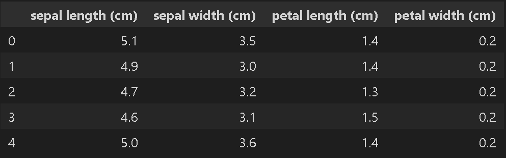
上記よりデータは4次元、ラベルは3種のカテゴリカルデータが150サンプルあることがわかります。
(参考:IRISのデータセット情報はUCI機械学習リポジトリで確認できます)
2-2.OpenMLから取得:fetch_openml
外部のOpenMLからサンプルデータセットを取得する場合は、「sklearn.datasets.fetch_openml」を使用します。sklearnのversionは0.20.以上となります。
APIは下記の通りです。
[API]
sklearn.datasets.fetch_openml(name: Optional[str] = None, *,
                              version: Union[str, int] = 'active',
                              data_id: Optional[int] = None,
                              data_home: Optional[Union[str, PathLike]] = None,
                              target_column: Optional[Union[str, List]] = 'default-target',
                              cache: bool = True,
                              return_X_y: bool = False,
                              as_frame: Union[str, bool] = 'auto',
                              n_retries: int = 3,
                              delay: float = 1.0,
                              parser: str = 'warn',
read_csv_kwargs: Optional[Dict] = None)[source]サンプルとしてMNISTのデータを取得しました。
[IN]
from sklearn.datasets import fetch_openml
mnist = fetch_openml('mnist_784', version=1, data_home="./data/", as_frame=False)  # data_home:保存先

# データの取り出し
X = mnist.data
y = mnist.target

plt.imshow(X[0].reshape(28, 28), cmap='gray')
print("この画像データのラベルは{}です".format(y[0]))

[OUT]
この画像データのラベルは5です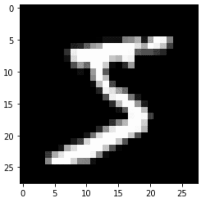
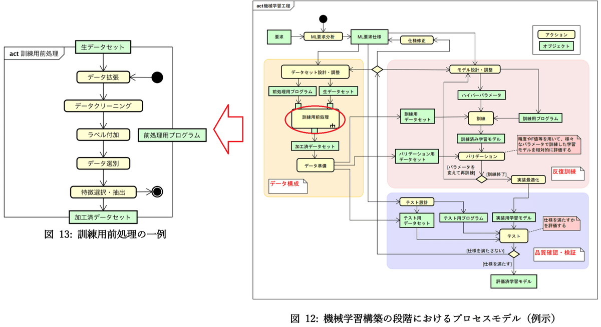
3.データの前処理
機械学習をする前には特徴量を作ったりデータを分けたりと学習前に処理することが多いです。本章では前処理を説明します。
3ー1.前処理1:正規化(Normalization)、標準化(Standardization)
例として線形モデルではスケールが大きいと回帰係数が小さくなり正則化がかかりにくくなるため学習がうまく進まないことがあります(変数同士のスケール差が大きいのもよくない)。
よって事前に正規化・標準化することが一般的です。
3-1-1.正規化、標準化の説明
【正規化】
正規化とはデータの最小値0, 最大値1にする処理です。
$$
正規化 = \frac{x-最小値x_{min}}{最大値x_{max}-最小値x_{min}}
$$
下記特徴があるため通常は標準化を使用します(画像データのように数値範囲が決まっているのであれば問題無い)。
【正規化の特徴】
●平均値が0にならないためモデルの学習にやや不利
●外れ値の影響を受けやすい。
import pandas as pd
import matplotlib.pyplot as plt
import numpy as np
import japanize_matplotlib

df = pd.DataFrame(datas, columns=columns_data)
df_min0 = df['sepal length (cm)']-df['sepal length (cm)'].min() #データの最小値を引くことで、更新後のデータ最小値が0になる。
plotdatas = [df['sepal length (cm)'], df_min0, df_min0/df_min0.max()]
titles = ['オリジナルデータ', '最小値を0に調整', '最大値を1に調整(正規化)']

plt.figure(figsize=(12,6))
for idx, _ in enumerate(zip(plotdatas, titles)):
   plotdata, title = _
   ax = plt.subplot(1,3,idx+1)
   plt.scatter(np.zeros_like(plotdata), plotdata)
   ax.set(title=title,
           xlabel='',
           ylabel='sepal length',
           ylim=[0,8],
           yticks=np.linspace(0,8,9))
   plt.grid()

plt.show()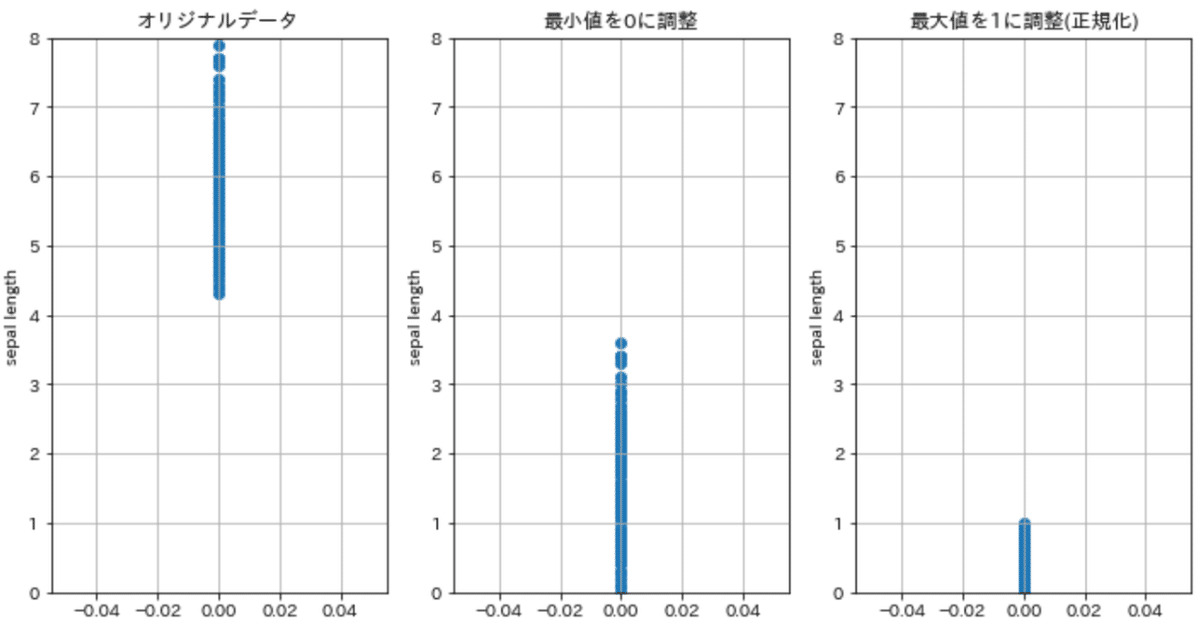
【標準化】
標準化は平均値0, 分散1にする処理です(下記イメージ)。
$$
標準化 = \frac{x-平均値μ}{標準偏差σ}
$$
[In]
df_mean = df['sepal length (cm)']-df['sepal length (cm)'].mean() #データの平均値を引くことで、更新後のデータ平均値が0になる。
plotdatas = [df['sepal length (cm)'], df_mean, df_mean/df_mean.std()]
titles = ['オリジナルデータ', '平均値を0に調整', '標準偏差を1に調整(標準化)']

plt.figure(figsize=(12,6))
for idx, _ in enumerate(zip(plotdatas, titles)):
   plotdata, title = _
   ax = plt.subplot(1,3,idx+1)
   plt.scatter(np.zeros_like(plotdata), plotdata)
   ax.set(title=title,
           xlabel='',
           ylabel='sepal length',
           ylim=[-2,8],
           yticks=np.linspace(-2,8,11))
   plt.grid()
plt.show()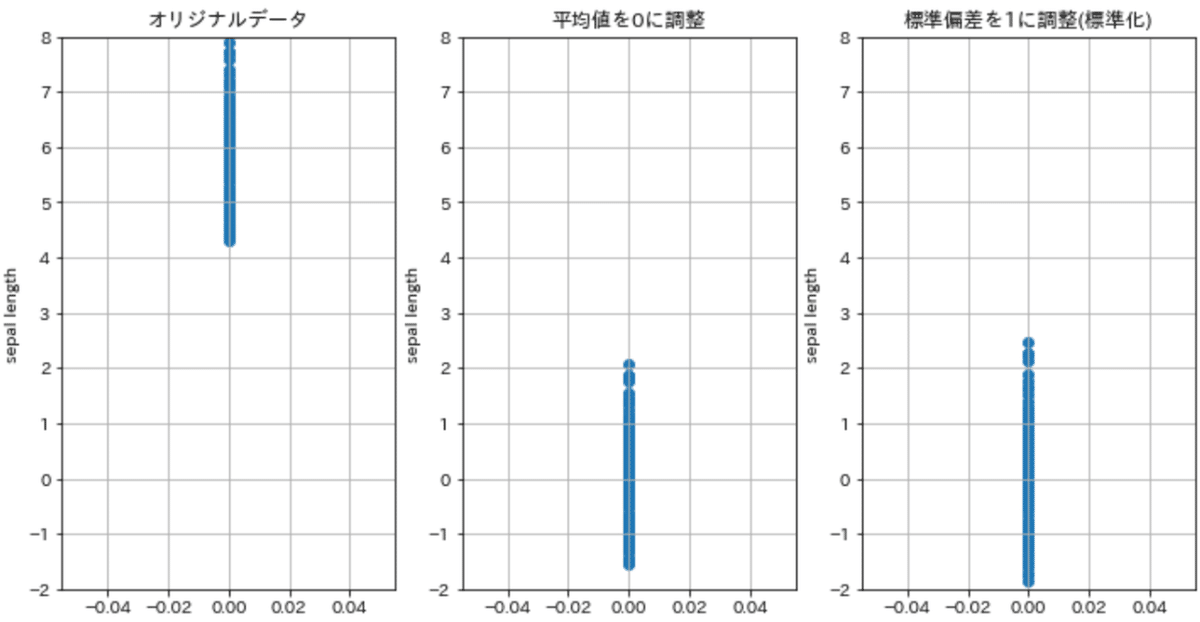
sklearnでは各次元に対して一括で正規化・標準化処理が可能です。
3-1-2.正規化の実装:MinMaxScaler()
正規化はMinMaxscaler()を使用して、fit()->transform()で処理可能です。
[In]
from sklearn.preprocessing import MinMaxScaler

minmaxscaler = MinMaxScaler()
minmaxscaler.fit(datas) #fitでmax, minを読み取り学習
datas_mm = minmaxscaler.transform(datas) #transformで学習した値から正規化※出力はnumpy.ndarray型
[Out] ※省略3-1-3.標準化の実装:StandardScaler()
標準化はStandardScaler()です。APIはMinMaxScaler()と同じです。下記の通りfit()->transform()はまとめてfit_transform()で処理可能です。
[In]
from sklearn.preprocessing import StandardScaler
stdscaler = StandardScaler()
datas_ss = stdscaler.fit_transform(datas)
3-1ー4.L2正規化:Normalizer()
L2ノルム(ユークリッドノルム)で割ることで特徴量を正規化できます。
例として各データ内にばらつきが大きい場合(画像データの場合は特徴量マップにおけるチャネル方向のばらつき)、結果がそのデータ(パラメータや入力値)に大きな影響を受ける可能性があるためL2Normで正規化します。
L2ノルムは別名「ユークリッド距離」とも呼ばれ2点間の距離は下記式で計算できます。
$$
d(A, B) =\sqrt{(x_{1}-x_{2})^{2}+(y_{1}-y_{2})^{2}} \\
Aのx,y座標=x_{1}, y_{1} \\
Bのx,y座標=x_{2}, y_{2}
$$
多次元におけるL2ノルムは下記式となり同一次元方向のユークリッド距離(norm)を求め、各値をnormで割ることで正規化します。これは「そのセルの値は標準値(L2ノルム)何個分か」を示す値となります。
$$
norm = \sqrt{x_1^2+x_2^2+\cdots+x_n^2}
$$
$$
正規化されたセルの値=\frac{セルの値}{norm}
$$
[In]
import numpy as np
from sklearn.preprocessing import Normalizer

array = np.array([[1,2,30]])
print(f'配列形状:{array.shape}')

normalizer = Normalizer() #L2ノルムで正規化
array_l2 = normalizer.fit_transform(array)
print(array_l2)

[OUT]
配列形状:(1, 3)
[[0.03324112 0.06648225 0.99723374]]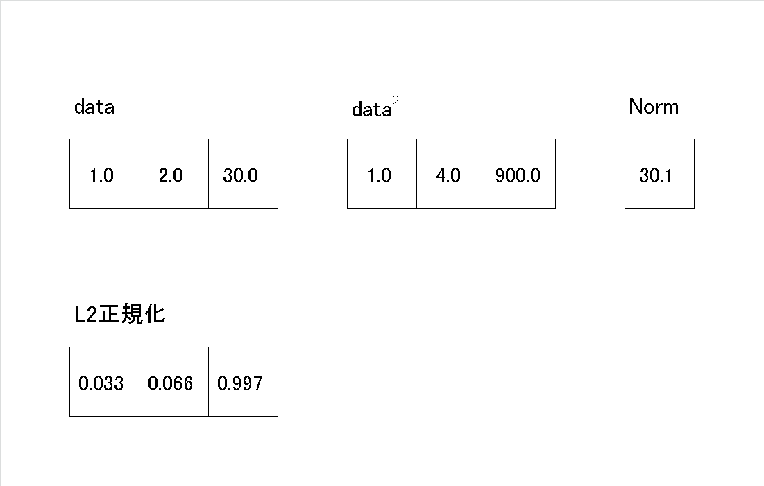
[IN]
array2 = np.array([[1, 2, 30],
                   [4, 5, 60],
                   [7, 8, 90]])

print(f'配列形状:{array2.shape}')
normalizer = Normalizer() #L2ノルムで正規化
array2_l2 = normalizer.fit_transform(array2)
print(array2_l2)

[OUT]
配列形状:(3, 3)
[[0.03324112 0.06648225 0.99723374]
 [0.06629025 0.08286281 0.99435374]
 [0.07724086 0.08827527 0.99309684]]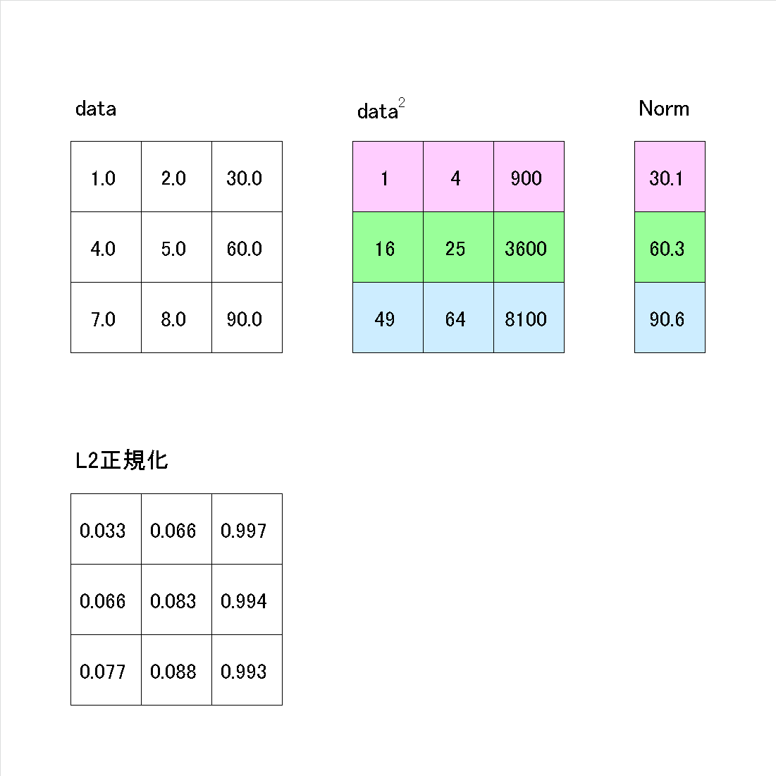
3-1-5.(参考)その他前処理
その他にも様々な前処理ができますので参考までに
●Box-Cox変換:PowerTransformer(methond='box-cox')
●Yeo-Johnson変換:PowerTransformer(methond='yeo-johnson')
●RankGauss:QuantileTransformer(n_quantiles, output_distribution)
3-2.前処理2:エンコーディング
エンコーディングはカテゴリカルデータのユニークな値と同じ数の次元を作成して該当する項目に1、それ以外を0にします。
3-2-1.One-Hotエンコーディング_Scikit-learn
One-Hotエンコーディングは下記の通りです。データの次元変換や.Aをつけたり覚えにくいです。
[In]
from sklearn.preprocessing import OneHotEncoder
OneHotEncoder().fit_transform(labels.reshape(-1,1)).A
[Out]
[[1. 0. 0.]
[1. 0. 0.]
・・以下省略
3-2-2.ダミーコーディング:pd.get_dummies
Pandasのget_dummiesを使用したら簡単に作成できます。drop_first=Trueにすると項目数を1つ減らして表現します。
[In]
df_label = pd.DataFrame(labels, columns=['label'])

irisidxname = dict(zip([0,1,2], columns_label)) #output->{0: 'setosa', 1: 'versicolor', 2: 'virginica'}
df_label['label'] = df_label['label'].map(irisidxname)
display(pd.get_dummies(df_label, prefix=['label'])) #全ラベルデータをエンコーディング
display(pd.get_dummies(df_label, prefix=['label'], drop_first=True)) #(全データ-1)の数をエンコーディング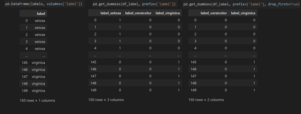
3-2-3.ラベルエンコーダー:LabelEncoder
LabelEncoderはカテゴリカルなデータに整数を割り当てます。またその整数から元のデータに復元することも可能です。
[In]
from sklearn.preprocessing import LabelEncoder

labelen = LabelEncoder() # LabelEncoder()をインスタンス化
df_label_1dim = df_label['label'].ravel() #1次元化->numpy.ndarray
labelen.fit(df_label['label'].ravel())

df_label_encoded = labelen.transform(df_label['label'].ravel())#エンコーディング
display(df_label_1dim ,df_label_encoded)

labelen.inverse_transform([0,1,2]) #インデックスからラベルを取得※デコーディング
[Out]
array(['setosa', 'setosa', 'setosa', 'setosa', 'setosa', 'setosa', 'setosa', 'setosa', 'setosa', 'setosa', 'setosa', 'setosa', 'setosa', 'setosa', 'setosa', 'setosa', 'setosa', 'setosa', 'setosa', 'setosa', 'setosa', 'setosa', 'setosa', 'setosa', 'setosa', 'setosa', 'setosa', 'setosa', 'setosa', 'setosa', 'setosa', 'setosa', 'setosa', 'setosa', 'setosa', 'setosa', 'setosa', 'setosa', 'setosa', 'setosa', 'setosa', 'setosa', 'setosa', 'setosa', 'setosa', 'setosa', 'setosa', 'setosa', 'setosa', 'setosa', 'versicolor', 'versicolor', 'versicolor', 'versicolor', 'versicolor', 'versicolor', 'versicolor', 'versicolor', 'versicolor', 'versicolor', 'versicolor', 'versicolor', 'versicolor', 'versicolor', 'versicolor', 'versicolor', 'versicolor', 'versicolor', 'versicolor', 'versicolor', 'versicolor', 'versicolor', 'versicolor', 'versicolor', 'versicolor', 'versicolor', 'versicolor', 'versicolor', 'versicolor', 'versicolor', 'versicolor', 'versicolor', 'versicolor', 'versicolor', 'versicolor', 'versicolor', 'versicolor', 'versicolor', 'versicolor', 'versicolor', 'versicolor', 'versicolor', 'versicolor', 'versicolor', 'versicolor', 'versicolor', 'versicolor', 'versicolor', 'versicolor', 'versicolor', 'virginica', 'virginica', 'virginica', 'virginica', 'virginica', 'virginica', 'virginica', 'virginica', 'virginica', 'virginica', 'virginica', 'virginica', 'virginica', 'virginica', 'virginica', 'virginica', 'virginica', 'virginica', 'virginica', 'virginica', 'virginica', 'virginica', 'virginica', 'virginica', 'virginica', 'virginica', 'virginica', 'virginica', 'virginica', 'virginica', 'virginica', 'virginica', 'virginica', 'virginica', 'virginica', 'virginica', 'virginica', 'virginica', 'virginica', 'virginica', 'virginica', 'virginica', 'virginica', 'virginica', 'virginica', 'virginica', 'virginica', 'virginica', 'virginica', 'virginica'], dtype=object)
array([0, 0, 0, 0, 0, 0, 0, 0, 0, 0, 0, 0, 0, 0, 0, 0, 0, 0, 0, 0, 0, 0, 0, 0, 0, 0, 0, 0, 0, 0, 0, 0, 0, 0, 0, 0, 0, 0, 0, 0, 0, 0, 0, 0, 0, 0, 0, 0, 0, 0, 1, 1, 1, 1, 1, 1, 1, 1, 1, 1, 1, 1, 1, 1, 1, 1, 1, 1, 1, 1, 1, 1, 1, 1, 1, 1, 1, 1, 1, 1, 1, 1, 1, 1, 1, 1, 1, 1, 1, 1, 1, 1, 1, 1, 1, 1, 1, 1, 1, 1, 2, 2, 2, 2, 2, 2, 2, 2, 2, 2, 2, 2, 2, 2, 2, 2, 2, 2, 2, 2, 2, 2, 2, 2, 2, 2, 2, 2, 2, 2, 2, 2, 2, 2, 2, 2, 2, 2, 2, 2, 2, 2, 2, 2, 2, 2, 2, 2, 2, 2])
array(['setosa', 'versicolor', 'virginica'], dtype=object)3-3.前処理3:特徴量作成
3-3-1.交互作用特徴量:PolynomialFeatures
機械学習=自動で特徴量を捉えるためデータを突っ込めば高精度が出る というわけではなく必要なデータ項目を作成・抽出してあげる必要があります。(Kaggle_titanic)
交互作用特徴量は各次元を掛け合わせることで新しい次元を作成します。
[In]
from sklearn.preprocessing import PolynomialFeatures
a = np.array([[1,10,100],[2,20,200],[3,30,300]])
a = pd.DataFrame(a, columns=['x','y','z'])
display(a)
b = PolynomialFeatures(include_bias=False).fit_transform(a)
pd.DataFrame(b, columns=['x','y','z','x^2','xy','xz','y^2','yz','z^2'])

[Out]左がa(処理前)、右がb(交互作用特徴量で処理)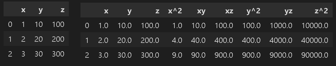
3-4.前処理4:データ分割
3-4-1.データの一括分割:train_test_split()
一般的に機械学習では学習用、検証用、テスト用データセットに分割して使用します。今回は学習・テスト用データに分割しており、データ分割はtrain_test_split()を使用します。
[In]
from sklearn import datasets
import pandas as pd
from sklearn.model_selection import train_test_split
iris = datasets.load_iris() #load_xxx()でデータやラベルなどを含む辞書型データを取得
datas, labels = iris.data, iris.target #データとラベル取得
df, df_label = pd.DataFrame(datas, columns=iris.feature_names), pd.DataFrame(labels, columns=['label'])
print(df.shape, df_label.shape)
x_train, x_test, y_train, y_test = train_test_split(df, df_label, test_size=0.25, random_state=0) #データとラベルを分割, test_size=テストデータの割合を指定, random_stateで乱数を固定
print(x_train.shape, x_test.shape, y_train.shape, y_test.shape)
[Out]
(150, 4) (150, 1)
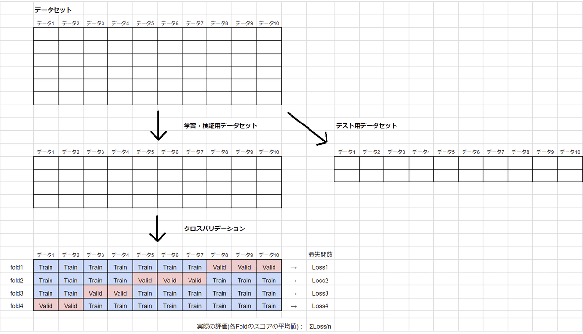
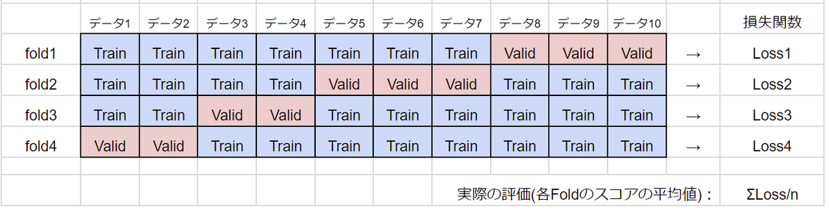
(112, 4) (38, 4) (112, 1) (38, 1)3-4-2.K分割交差検証:KFold()
K-分割交差検証は指定した回数分だけデータ分割を全データ分で繰り返します。機械学習では各Foldを平均化することで汎化性を高めます(下図出典)。
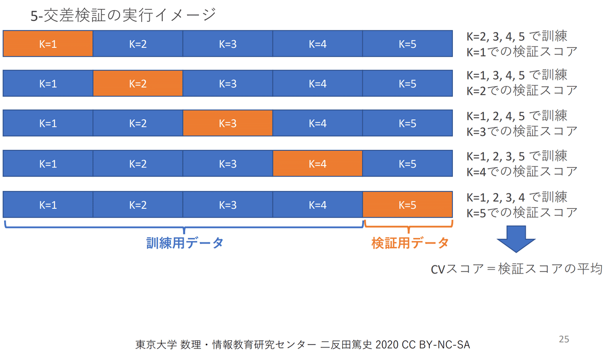
クロスバリデーションはKFold(分割数)で作成してFor分で回します。
[In]
from sklearn.model_selection import KFold

df_small = df[:10]
kf = KFold(n_splits=4, shuffle=True, random_state=0)
for train_idx, val_idx in kf.split(df_small):
    print('train_idx:', train_idx, 'val_idx:', val_idx)
    display(df_small.iloc[train_idx]) #indexからデータを取得
    display(df_small.iloc[val_idx]) #indexからデータを取得
[Out] ※displayでのDataframeの表示は省略
train_idx: [0 1 3 5 6 7 9] val_idx: [2 4 8]
train_idx: [0 2 3 4 5 7 8] val_idx: [1 6 9]
train_idx: [0 1 2 4 5 6 8 9] val_idx: [3 7]
train_idx: [1 2 3 4 6 7 8 9] val_idx: [0 5]3-4-3.グループK分割交差検証:GroupKFold
K分割交差検証ではランダムにデータを分割して一部を検証データ、残りを学習データとしました。これは下記のような条件では問題となります。
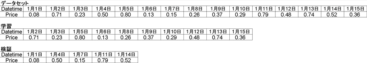
【例1:時系列データ】
時系列データをランダムに分割すると最新日付のデータが学習に使われる可能性があります。この場合未来の(最新)データで学習して、過去の(古い)データで検証することとなります。
つまり未来のデータを予想するのが目的のタスクで未来のデータを使用して過去を推論するため一種のチーティングをしておりスコアが過剰に上がる(検証性の信頼性が低くなる)可能性があります。
【例2:グルーピングされたデータ内で高い相関がある場合】
K分割交差検証の目的は「機械学習モデルの過学習防止」です。もし分割した学習データと検証データが似たようなデータ(高い相関がある)の場合、機械学習モデルは学習したデータと類似の問題を計算するだけのため簡単に高い性能を出すことが出来ます。つまり高い相関があるデータのグループが学習と訓練に混ざると過学習を生じやすくなります。
一般的にグループデータ(例:クラスタリングされたデータ、医療での患者ごとのデータ、各センサーのデータなど)は類似性をもっているため、同一グループのデータが学習と訓練に混ざると簡単に高い性能を出すことが出来る(学習に使用した類似データが検証にも孫算するため)ため、過学習を生じやすくなります。
グループ内の類似性による過学習を防止するための手法としてグループK分割交差検証があります。なおデータの構造がシンプルでデータ間に強い相関がない場合や、グループ構造が不明または不確かな場合、また計算コストを下げたい場合などはK分割交差検証を実施します。
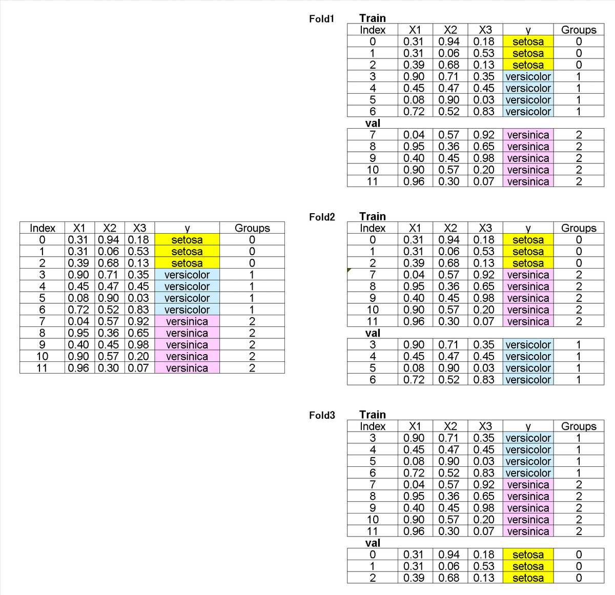
グループK分割交差検証(fold=3)の概要は下記の通りです。
データセットの中にグループを割り当てる※引数に渡すgroupsは数値でも文字列(カテゴリカル)でもどちらでもよい
分割する時に指定したグループがTrain/Valのどちらかにしか所属しないようにする。つまりグループをひと固まりとみなして分割する。
上記分割手法のため、等分割にはならない
参考として、1データ(1行)のことをデータポイントと呼ぶ
次にコードを実装します。まずは適当なデータとしてIrisを使用します。
[IN]
import pandas as pd
import numpy as np
from sklearn import datasets
from sklearn.model_selection import train_test_split, KFold, GroupKFold

iris = datasets.load_iris()
datas, targets = iris.data, iris.target
df_iris = pd.DataFrame(datas, columns=iris.feature_names)
label2name = {0: 'setosa', 1: 'versicolor', 2: 'virginica'} #ラベル値 ->ラベル名の辞書
df_iris['target'] = pd.Series(targets).map(label2name) #ラベル値 ->ラベル名に変換

# クラスごとにデータを抽出し、12個のデータセットを作成(setosa:3個, versicolor:4個, virginica:5個)
df_sampled = df_iris[df_iris['target'] == label2name[0]].iloc[:3].append(
    [df_iris[df_iris['target'] == label2name[1]].iloc[:4],
     df_iris[df_iris['target'] == label2name[2]].iloc[:5]])

display(df_sampled)

[OUT]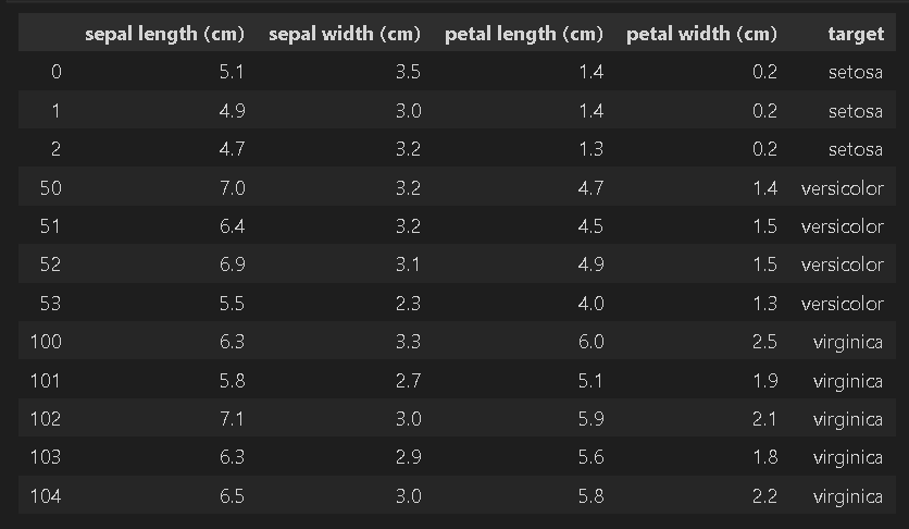
グループK分割交差検証は”gkf = GroupKFold(n_splits=<分割数>)”でインスタンスを作成後、”gkf.split(X=<データ>, group=<グループが判断できる配列> )”を渡します。
[API]
sklearn.model_selection.GroupKFold(n_splits=5)

[API]
split(X, y=None, groups=None)GroupKFoldの出力はジェネレーターでありlist(<出力>)によりリストとして取得可能
1つの出力は(<Trainのindex番号>, <Trainのindex番号>)となっている。
1つのグループは必ずTrain/Valのどちらかにしか属していない
動作原理上$${グループ数>=n分割数}$$でないとエラー
[IN]
# グループラベルを割り当てる
groups = [0, 0, 0, 1, 1, 1, 1, 2, 2, 2, 2, 2]

# 特徴量とターゲットを抽出
X = df_sampled.drop('target', axis=1).values
y = df_sampled['target'].values

# GroupKFoldでデータを分割
gkf = GroupKFold(n_splits=3) #n_splitsは分割数 ※「グループ数>=分割数」でないとエラーになる
splits = list(gkf.split(X, y, groups))
print(gkf.split(X, y, groups)) #GroupKFoldの返り値 :ジェネレーター->listに変換
print(splits, end='\n\n')


# 各分割で学習データと検証データを表示
for i, (train_index, test_index) in enumerate(splits):
    print(f"Split {i + 1}")
    print("Train Index:", train_index, ", Test Index:", test_index)
    print(f'Test data:{y[test_index]}')
    print(f'{"#"*100}')
[OUT]
<generator object _BaseKFold.split at 0x00000224155C05F0>
[(array([0, 1, 2, 3, 4, 5, 6]), array([ 7,  8,  9, 10, 11])),
(array([ 0,  1,  2,  7,  8,  9, 10, 11]), array([3, 4, 5, 6])),
(array([ 3,  4,  5,  6,  7,  8,  9, 10, 11]), array([0, 1, 2]))]

Split 1
Train Index: [0 1 2 3 4 5 6] , Test Index: [ 7  8  9 10 11]
Test data:['virginica' 'virginica' 'virginica' 'virginica' 'virginica']
####################################################################################################
Split 2
Train Index: [ 0  1  2  7  8  9 10 11] , Test Index: [3 4 5 6]
Test data:['versicolor' 'versicolor' 'versicolor' 'versicolor']
####################################################################################################
Split 3
Train Index: [ 3  4  5  6  7  8  9 10 11] , Test Index: [0 1 2]
Test data:['setosa' 'setosa' 'setosa']
####################################################################################################
①グループは文字列でも問題ない、②出力はindexのため渡すデータはXのみでよい、③グループ数>=n分割数であれば値は等しくなくてよい ので条件を変えて実行しました。
今回は12データを6グループで4分割しました。KFoldだと各Foldのデータ数は3になりますが、今回はグループ分けしているため(4,4,2,2)となり、Train/Valでデータが分離されていることが確認できました。
[IN]
# グループラベルを割り当てる
groups = ['A', 'A', 'B', 'B', 'C', 'C', 'D', 'D', 'E', 'E', 'F', 'F']

# 特徴量とターゲットを抽出
X = df_sampled.drop('target', axis=1).values
y = df_sampled['target'].values

# GroupKFoldでデータを分割
gkf = GroupKFold(n_splits=4) #n_splitsは分割数 ※「グループ数>=分割数」でないとエラーになる
splits = list(gkf.split(X=X, groups=groups))
print(splits, end='\n\n')


# 各分割で学習データと検証データを表示
for i, (train_index, test_index) in enumerate(splits):
    print(f"Split {i + 1}")
    print("Train Index:", train_index, ", Test Index:", test_index)
    print(f'Test data:{y[test_index]}')
    print(f'{"#"*100}')
[OUT]
Split 1
Train Index: [0 1 4 5 6 7 8 9] , Test Index: [ 2  3 10 11]
Test data:['setosa' 'versicolor' 'virginica' 'virginica']
####################################################################################################
Split 2
Train Index: [ 2  3  4  5  6  7 10 11] , Test Index: [0 1 8 9]
Test data:['setosa' 'setosa' 'virginica' 'virginica']
####################################################################################################
Split 3
Train Index: [ 0  1  2  3  4  5  8  9 10 11] , Test Index: [6 7]
Test data:['versicolor' 'virginica']
####################################################################################################
Split 4
Train Index: [ 0  1  2  3  6  7  8  9 10 11] , Test Index: [4 5]
Test data:['versicolor' 'versicolor']
####################################################################################################
4.教師無し学習
4-1.主成分分析:PCA
主成分分析とは複数ある次元を圧縮して強い特徴を持つ次元に変換します。高次元を1~3次元に圧縮するとグラフ化による可視化が可能です。
irisデータは['sepal length','sepal width ','petal length ','petal width']の4つの次元を持ちますが参考として2次元に変換してみます。主成分分析の前には標準化が必要であり、参考として標準化前後の比較を作成しました。
[In]
from sklearn.decomposition import PCA #PCAで特徴量を削減
from sklearn.preprocessing import StandardScaler
import seaborn as sns

#標準化前
pca = PCA(n_components=2) #n_componentsで削減する特徴量の数を指定
pca.fit(df) #fitで特徴量を抽出
df_pca = pca.transform(df) #transformで特徴量を抽出
df_pca = pd.DataFrame(df_pca, columns=['pca1','pca2'])
print('各次元での寄与率(標準化前)', pca.explained_variance_ratio_) #各次元での寄与率

#標準化後
df_ss = StandardScaler().fit_transform(df) #output->numpy.ndarray型
pca_ss = PCA(n_components=2) #n_componentsで削減する特徴量の数を指定
df_pca_ss = pca_ss.fit_transform(df_ss) #fitで特徴量を抽出
df_pca_ss = pd.DataFrame(df_pca_ss, columns=['pca1','pca2'])
print('各次元での寄与率(標準化後)', pca_ss.explained_variance_ratio_) #各次元での寄与率

#グラフ化の前処理
plt.rcParams['font.size'] = 14
labelnames = [irisidxname[i] for i in labels] #{0: 'setosa', 1: 'versicolor', 2: 'virginica'}から数値をラベル化
fig = plt.figure(figsize=(20,8))
#グラフ_標準化前
ax = plt.subplot(1,2,1)
sns.scatterplot(x='pca1', y='pca2', data=df_pca, s=80,
               hue=labelnames, style=labelnames, palette='Set1')
ax.set_title(f'主成分分析による2次元化(標準化前)')
plt.grid()
#グラフ_標準化後
ax = plt.subplot(1,2,2)
sns.scatterplot(x='pca1', y='pca2', data=df_pca_ss, s=80,
               hue=labelnames, style=labelnames, palette='Set1')
ax.set_title(f'主成分分析による2次元化(標準化前)')
plt.grid()
plt.show()

[Out]
各次元での寄与率(標準化前) [0.92461872 0.05306648]
各次元での寄与率(標準化後) [0.72962445 0.22850762]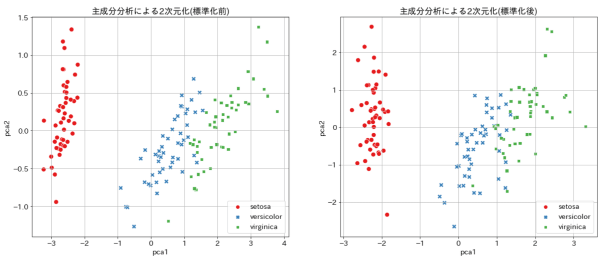
4-2.クラスタリング(k-平均法):KMeans
クラスタリングとはデータの重心からの距離を計算することでデータをグループ分けしてくれる手法です。使用時にはデータを何種類に分類するかを指定する必要があります。
先ほどの主成分分析から得られた2次元データを使用して正解ラベルを予想し、正解値と比較してみます。
[In]
from sklearn.cluster import KMeans
kmeans = KMeans(n_clusters=3, random_state=0).fit(df_pca_ss) #random_stateで乱数を固定
print('クラスタの中心', kmeans.cluster_centers_, '形状', kmeans.cluster_centers_.shape) #クラスタの中心

clusters = kmeans.predict(df_pca_ss) #クラスタリング結果を取得


#グラフ_標準化後:正解データ
fig = plt.figure(figsize=(20,8))
ax = plt.subplot(1,2,1)
sns.scatterplot(x='pca1', y='pca2', data=df_pca_ss, s=80,
               hue=labelnames, style=labelnames, palette='Set1')
ax.set_title(f'主成分分析による2次元化(標準化後):正解データ')
plt.grid()
#グラフ_主成分分析+k-meansから予測したデータ
ax = plt.subplot(1,2,2)
sns.scatterplot(x='pca1', y='pca2', data=df_pca_ss, s=80,
               hue=clusters, style=clusters, palette='Set1')
ax.set_title(f'標準化後の主成分データからクラスタリングで正解値を予測')
plt.grid()
plt.show()

[Out]
クラスタの中心 [[-2.22  0.289] [ 0.572 -0.807] [ 1.72 0.603]] 形状 (3, 2)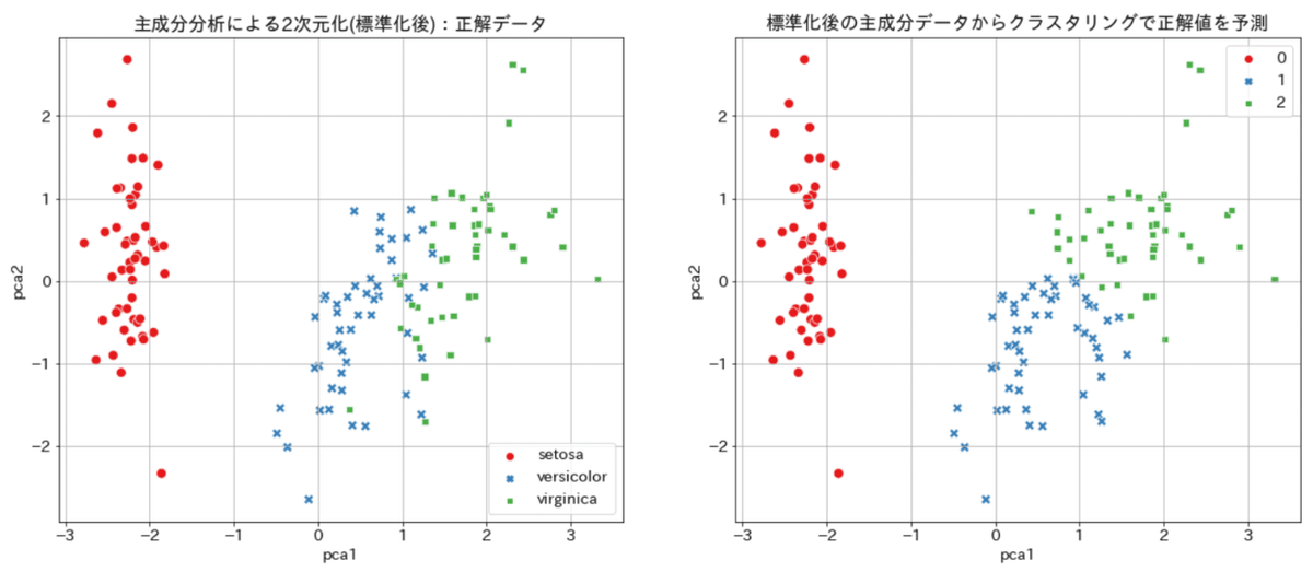
結果はsetosaは完璧ですが、versi.とvirgi.の境界部分がいまいちでした。
今回正解のグルーピングが3種類と分かっているため指定しましたが、わからないことも多いため状況に応じて決める必要があります。
5.スコア確認
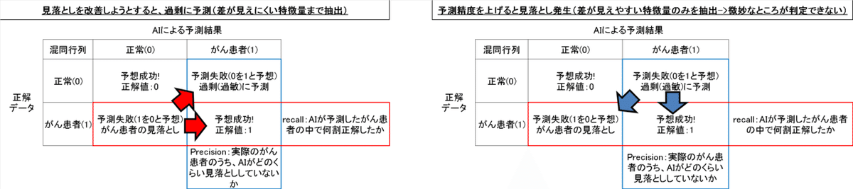
5-1.混同行列(Confusion Matrix)
【混同行列とは】
混合行列は2値分類における結果検証で使用されます。参考としてがん診断を想定して用語を自分なりに解釈すると下記の通りです。
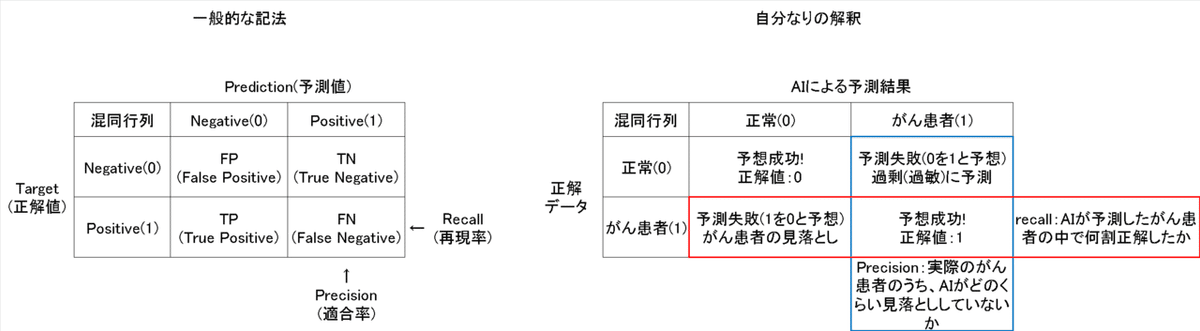
●Accuracy(精度):いわゆる正確さであり、正解値/全データで計算される。ただし2値データの片方のデータが多い場合は全予測を正常と予測するだけで高精度になるため評価指標としては不適です。
●Precision(適合率):AIが2値における予測したい方の結果に対してどれくらいの割合で予測できたかを判断する。ただし予測の見落としは判断できない。
●recall(再現率):AIが2値における予測したい方の結果に対してどれくらい見落としがないかを判断する。ただし過敏な予測は判断できない。
●f1score:Precisionとrecallを総合的に評価
Precisionとrecallのイメージは下記の通りです。
【コーディング】
コードは下記の通りです。参考までに3値分類ですがpresicion, recall, f1スコアも計算してみます。
[In]
from sklearn.metrics import confusion_matrix, precision_score, recall_score, f1_score
matrix = confusion_matrix(labels, clusters)
print(matrix)
[Out]
[[50  0  0]
[ 0 39 11]
[ 0 14 36]]

[In]
precision = precision_score(labels, clusters, average='micro')
recall = recall_score(labels, clusters, average='micro')
f1score = f1_score(labels, clusters, average='micro')
print(precision, recall, f1score)
[Out]
0.8333333333333334 0.8333333333333334 0.8333333333333334
混同行列の結果を可視化すると下記の通りです。
[In]
fig, ax = plt.subplots(figsize=(8,6))
sns.heatmap(matrix, annot=True, fmt='d', cmap='Blues', cbar=False, #fmt='d'で整数
       xticklabels=iris.target_names, yticklabels=iris.target_names)
ax.set(title='confusion matrix', ylabel='True label', xlabel='Predicted label')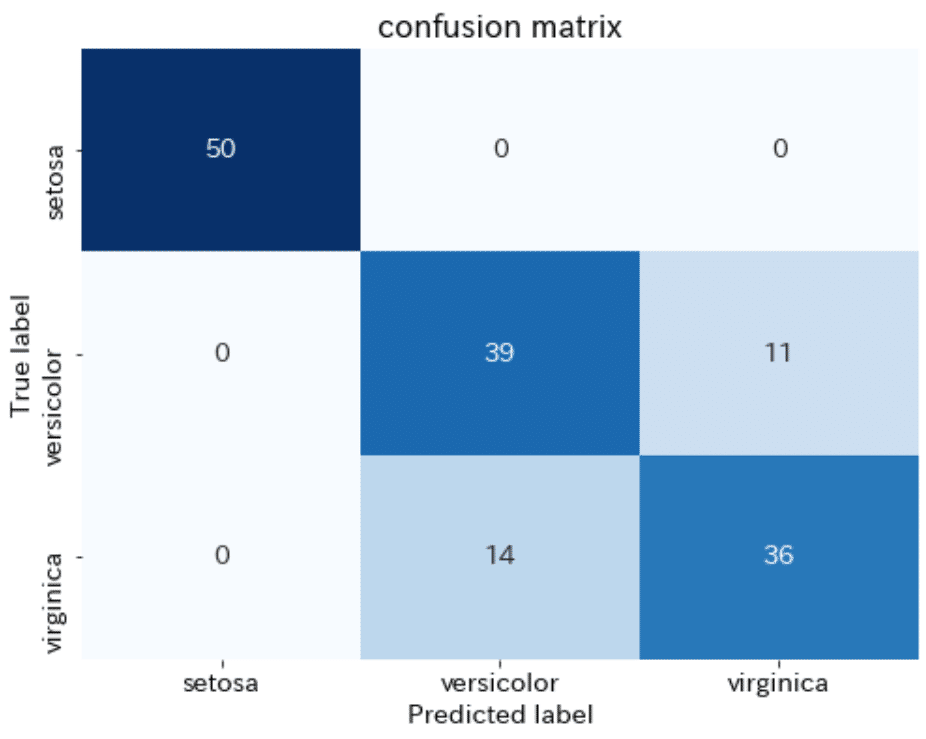
6.ハイパーパラメータの調整
機械学習ではすべての特徴量を自動で取得はできません。よって人がモデルの最適な値を調整する必要があり、調整値をハイパーパラメータと呼びます。
6-1.GRID SEARCH
複数のハイパーパラメータを試行して最適な値を見つける手法をGrid searchといいます。まずは参考として通常通りにモデルを作成します。
●モデル用データ:sklearnのbreast_cancer(乳がんかどうかを判定)
●機械学習モデル:Random Forest Classifier(公式サイト)
●データ数:569
●データ分割:学習:56%, 検証:24%、テスト:20%に分割
[In]
from sklearn.tree import DecisionTreeClassifier
from sklearn import datasets
from sklearn.model_selection import train_test_split
from sklearn.model_selection import GridSearchCV

#Datasetsからデータを取得して、PandasでDataFrameに変換
cancer = datasets.load_breast_cancer()
datas, labels = cancer.data, cancer.target #データとラベル取得
columns_data, columns_label  = cancer.feature_names, cancer.target_names#データのカラム名とラベルのカラム名を取得
df_data = pd.DataFrame(datas, columns=columns_data) #データセット
df_label = pd.DataFrame(labels, columns=['target']) #ラベルデータ
# display(df_data.head()); display(df_label.head()) #データの表示

#データの分割
x_train_val, x_test, t_train_val, t_test = train_test_split(df_data, df_label, test_size=0.2, random_state=0) #学習・検証用データとテストデータへの分割:testデータは20%
x_train, x_val, t_train, t_val = train_test_split(x_train_val, t_train_val, test_size=0.3, random_state=0) #学習データは80%×0.7=56%, 検証データは80%×0.3=24%
print('x_train:', x_train.shape, 'x_val:', x_val.shape, 'x_test:', x_test.shape, 't_train:', t_train.shape, 't_val:', t_val.shape, 't_test:', t_test.shape)

#モデルの作成・学習・評価※通常処理
model = DecisionTreeClassifier(random_state=0) #モデルの作成
model.fit(x_train, t_train) #Trainデータを使用して学習
print(f'Train score:{model.score(x_train, t_train):.3f},Val score:{model.score(x_val, t_val):.3f}, Test score:{model.score(x_test, t_test):.3f}') #学習結果の評価
[Out]
x_train: (318, 30) x_val: (137, 30) x_test: (114, 30) t_train: (318, 1) t_val: (137, 1) t_test: (114, 1)
Train score:1.000,Val score:0.891, Test score:0.9476-1-1.実装1:ハイパーパラメータの確認
初めに(サイトから)調整できるハイパーパラメータを確認して範囲をしています。今回はRandom forestの"max_depth"と"min_samples_split"を5種ずつ試してみます。参考として下記に試行パターンを示します。
[In]
import itertools
import pandas as pd

params =[{
    'max_depth': [2,5,10,15,20],
    'min_samples_split': [2,5,10,15,20],}]

params_combi = itertools.product(params[0]['max_depth'], params[0]['min_samples_split']) #パラメータの設定を組み合わせたリストを作成
depths, splits = [], [] #木の深さと木を分割するためのサンプル数を格納するリストを作成
[(depths.append(i), splits.append(j)) for i, j in params_combi] #params_combiのパラメータをdepths, splitsに格納

pd.DataFrame([depths, splits], index=['max_depth','min_samples_split'], columns=[f'試行{i}' for i in range(25)])
[Out]
			試行0	試行1	試行2	試行3	試行4	試行5	試行6	試行7	試行8	試行9	試行10	試行11	試行12	試行13	試行14	試行15	試行16	試行17	試行18	試行19	試行20	試行21	試行22	試行23	試行24
max_depth		2	2	2	2	2	5	5	5	5	5	10	10	10	10	10	15	15	15	15	15	20	20	20	20	20
min_samples_split	2	5	10	15	20	2	5	10	15	20	2	5	10	15	20	2	5	10	15	20	2	5	10	15	20
6-1-2.グリッドサーチでの学習
①各ハイパーパラメータの値をリストで格納、②交差検証の分割数を指定、③学習、④結果の確認します。
[In]
#グリッドサーチでハイパーパラメータの調整
params =[{
    'max_depth': [2,5,10,15,20],
    'min_samples_split': [2,5,10,15,20],
}] #ハイパーパラメータの設定:max_depthは木の深さ、min_samples_splitは木を分割するためのサンプル数
cv = 5 #クロスバリデーションの分割数を指定

model = DecisionTreeClassifier(random_state=0) #モデルの作成
models_CV = GridSearchCV(estimator=model, param_grid=params, cv=cv, return_train_score=False) #グリッドサーチの実行

models_CV.fit(x_train_val, t_train_val) #学習・検証データを使用して学習
display(pd.DataFrame(models_CV.cv_results_).T) #学習結果の表示:計5×5=25回の試行で、最適なパラメータはどれか[Out]
0 1 2 3 4 5 6 7 8 9 10 11 12 13 14 15 16 17 18 19 20 21 22 23 24
mean_fit_time 0.003 0.003 0.003 0.003 0.003 0.004 0 0.006 0 0.006 0.004 0.004 0.004 0.004 0.005 0.005 0 0.003 0.005 0.002 0.003 0.006 0.004 0.004 0.004
std_fit_time 0 0 0 0.001 0 0 0 0.008 0 0.008 0.001 0.001 0 0.001 0.007 0.006 0 0.006 0.006 0.002 0.006 0.005 0 0.001 0
mean_score_time 0.001 0.001 0.001 0.001 0 0.001 0.003 0 0 0 0.001 0.001 0.001 0.001 0 0 0 0 0 0.003 0 0 0.001 0.001 0.001
std_score_time 0 0 0 0 0 0 0.006 0 0 0 0 0 0 0 0 0 0 0 0.001 0.006 0 0 0 0 0
param_max_depth 2 2 2 2 2 5 5 5 5 5 10 10 10 10 10 15 15 15 15 15 20 20 20 20 20
param_min_samples_split 2 5 10 15 20 2 5 10 15 20 2 5 10 15 20 2 5 10 15 20 2 5 10 15 20
params {'max_depth': 2, 'min_samples_split': 2} {'max_depth': 2, 'min_samples_split': 5} {'max_depth': 2, 'min_samples_split': 10} {'max_depth': 2, 'min_samples_split': 15} {'max_depth': 2, 'min_samples_split': 20} {'max_depth': 5, 'min_samples_split': 2} {'max_depth': 5, 'min_samples_split': 5} {'max_depth': 5, 'min_samples_split': 10} {'max_depth': 5, 'min_samples_split': 15} {'max_depth': 5, 'min_samples_split': 20} {'max_depth': 10, 'min_samples_split': 2} {'max_depth': 10, 'min_samples_split': 5} {'max_depth': 10, 'min_samples_split': 10} {'max_depth': 10, 'min_samples_split': 15} {'max_depth': 10, 'min_samples_split': 20} {'max_depth': 15, 'min_samples_split': 2} {'max_depth': 15, 'min_samples_split': 5} {'max_depth': 15, 'min_samples_split': 10} {'max_depth': 15, 'min_samples_split': 15} {'max_depth': 15, 'min_samples_split': 20} {'max_depth': 20, 'min_samples_split': 2} {'max_depth': 20, 'min_samples_split': 5} {'max_depth': 20, 'min_samples_split': 10} {'max_depth': 20, 'min_samples_split': 15} {'max_depth': 20, 'min_samples_split': 20}
split0_test_score 0.923 0.923 0.923 0.923 0.923 0.89 0.923 0.912 0.912 0.934 0.879 0.868 0.879 0.912 0.934 0.879 0.868 0.879 0.912 0.934 0.879 0.868 0.879 0.912 0.934
split1_test_score 0.945 0.945 0.945 0.945 0.945 0.923 0.912 0.901 0.945 0.901 0.912 0.923 0.923 0.945 0.901 0.912 0.923 0.923 0.945 0.901 0.912 0.923 0.923 0.945 0.901
split2_test_score 0.901 0.901 0.901 0.901 0.901 0.89 0.89 0.89 0.89 0.89 0.89 0.901 0.89 0.89 0.89 0.89 0.901 0.89 0.89 0.89 0.89 0.901 0.89 0.89 0.89
split3_test_score 0.923 0.923 0.923 0.923 0.923 0.934 0.934 0.934 0.934 0.912 0.923 0.934 0.923 0.945 0.901 0.923 0.934 0.923 0.945 0.901 0.923 0.934 0.923 0.945 0.901
split4_test_score 0.923 0.923 0.923 0.923 0.923 0.956 0.956 0.956 0.956 0.945 0.956 0.956 0.945 0.956 0.945 0.956 0.956 0.945 0.956 0.945 0.956 0.956 0.945 0.956 0.945
mean_test_score 0.923 0.923 0.923 0.923 0.923 0.919 0.923 0.919 0.927 0.916 0.912 0.916 0.912 0.93 0.914 0.912 0.916 0.912 0.93 0.914 0.912 0.916 0.912 0.93 0.914
std_test_score 0.014 0.014 0.014 0.014 0.014 0.026 0.022 0.024 0.024 0.02 0.027 0.03 0.024 0.025 0.021 0.027 0.03 0.024 0.025 0.021 0.027 0.03 0.024 0.025 0.021
rank_test_score 5 5 5 5 5 11 5 11 4 16 23 13 20 1 17 23 13 20 1 17 23 13 20 1 17またRandom forestのような木構造モデルではどの特徴量が性能に大きな影響を与えているかを可視化できます。
[In]
import matplotlib.pyplot as plt

plt.figure(figsize=(12,8))
plt.barh(y=cancer.feature_names, width=model.feature_importances_)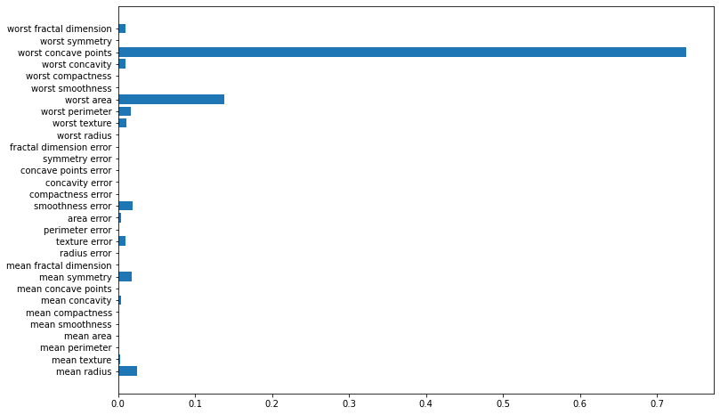
[In]
import graphviz
from sklearn.tree import export_graphviz

dot_data = export_graphviz(model)
graphviz.Source(dot_data)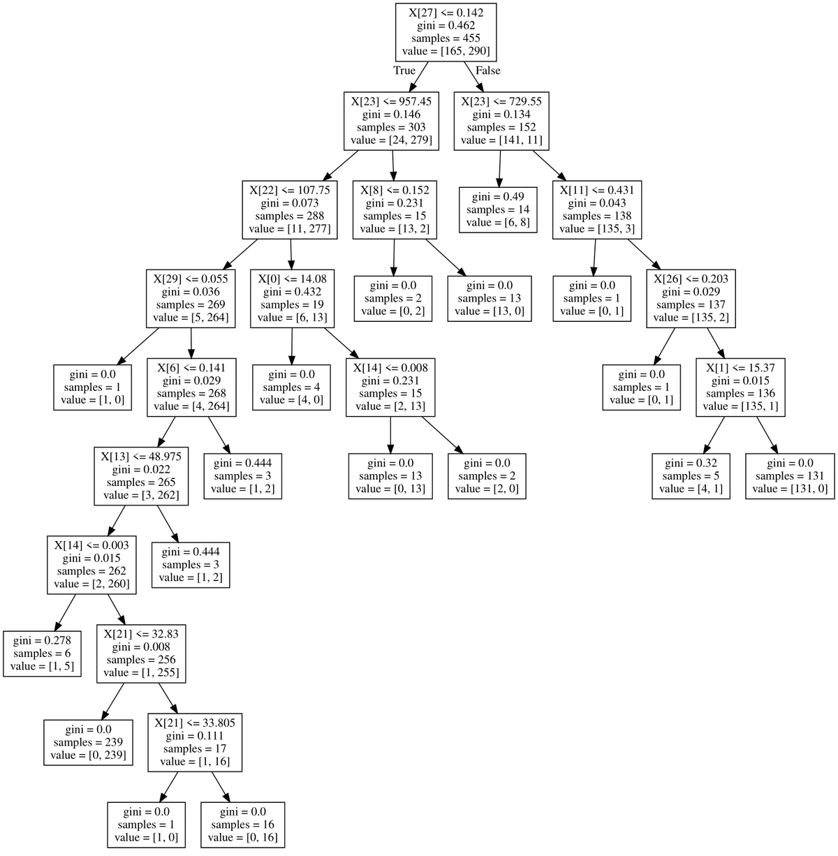
6-1-3.最適モデルの引継ぎ
グリッドサーチで最も精度がよかったモデルを引き継ぎます。今回の結果はテストデータがふつうにやるより悪くなっているためハイパーパラメータの検索範囲がいまいちだったことがわかります=>範囲を広げて再試行。
[In]
models_CV.best_params_ #最適なパラメータを確認
model = models_CV.best_estimator_ #最適なパラメータを使用してモデルを作成
print(model) #最適なパラメータを使用したモデルの表示
print(f'Train score:{model.score(x_train, t_train):.3f},Val score:{model.score(x_val, t_val):.3f}, Test score:{model.score(x_test, t_test):.3f}') #学習結果の評価[Out]
DecisionTreeClassifier(max_depth=10, min_samples_split=15, random_state=0)
Train score:0.972,Val score:0.993, Test score:0.904参考資料
https://www.ai-gakkai.or.jp/resource/aimap/
あとがき
私は機械学習する時に勾配ブースティング(XGboostやLightGBM)やPyTorchを使用しているためscikit-learnでの機械学習実装ではなく前処理やスコア評価の方に力を入れました。
ただ複数モデルをサクッとまとめて処理することもできるみたいなので、もっと勉強したいです。
それにしても見える化するためのグラフのコードの方が多いな・・・
この記事が気に入ったらサポートをしてみませんか?