
機械学習:R言語(Tidymodels)チュートリアルの和訳③

Bootstrap resampling and tidy regression models
ブートストラップ再サンプリングと回帰モデル
ブートストラップは、データセットを置換を伴ってランダムにサンプリングし、それぞれのブートストラップレプリケートに対して個別に分析を行う手法です。得られた推定値の変動は、我々の推定値の分散の合理的な近似となります。
library(tidymodels)ggplot(mtcars, aes(mpg, wt)) +
geom_point()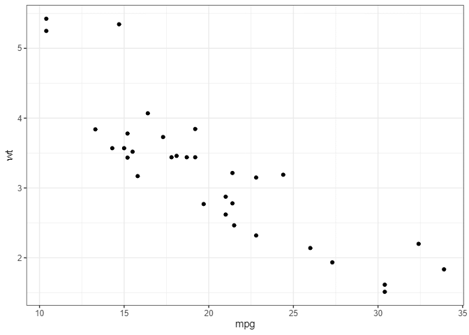
非線形最小二乗法(nls())でモデリングしてみます。
nlsfit <- nls(mpg ~ k / wt + b, mtcars, start = list(k = 1, b = 0))
summary(nlsfit)
#>
#> Formula: mpg ~ k/wt + b
#>
#> Parameters:
#>   Estimate Std. Error t value Pr(>|t|)
#> k   45.829      4.249  10.786 7.64e-12 ***
#> b    4.386      1.536   2.855  0.00774 **
#> ---
#> Signif. codes:  0 '' 0.001 '' 0.01 '' 0.05 '.' 0.1 ' ' 1
#>
#> Residual standard error: 2.774 on 30 degrees of freedom
#>
#> Number of iterations to convergence: 1
#> Achieved convergence tolerance: 6.813e-09
ggplot(mtcars, aes(wt, mpg)) +
geom_point() +
geom_line(aes(y = predict(nlsfit)))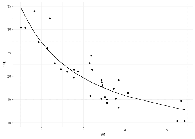
ブートストラップは、パラメータのp値と信頼区間を提供する一方で、モデルの仮定が実際のデータに当てはまらない場合でも、より頑健な信頼区間と予測を提供するための一般的な方法です。ブートストラップを使用することで、データの性質に対してより柔軟に対応できます。
ブートストラッピングモデル
rsample パッケージの bootstraps() 関数を使用して、ブートストラップレプリケートを生成することができます。まず、2000回のブートストラップレプリケートを構築します。各レプリケートは、置換を伴うランダムサンプリングによって得られます。生成されたオブジェクトは rset であり、これは rsplit オブジェクトの列を持つデータフレームです。
rsplit オブジェクトには主に2つのコンポーネントがあります:分析データセットと評価データセットで、それぞれ analysis(rsplit) と assessment(rsplit) でアクセスできます。ブートストラップサンプルの場合、分析データセットはブートストラップサンプル自体であり、評価データセットはアウトオブバッグ(OOB)サンプルから構成されます。
set.seed(27)
boots <- bootstraps(mtcars, times = 2000, apparent = TRUE)
boots
#> # Bootstrap sampling with apparent sample
#> # A tibble: 2,001 × 2
#>    splits          id
#>    <list>          <chr>
#>  1 <split [32/13]> Bootstrap0001
#>  2 <split [32/10]> Bootstrap0002
#>  3 <split [32/13]> Bootstrap0003
#>  4 <split [32/11]> Bootstrap0004
#>  5 <split [32/9]>  Bootstrap0005
#>  6 <split [32/10]> Bootstrap0006
#>  7 <split [32/11]> Bootstrap0007
#>  8 <split [32/13]> Bootstrap0008
#>  9 <split [32/11]> Bootstrap0009
#> 10 <split [32/11]> Bootstrap0010
#> # ℹ 1,991 more rows
ブートストラップサンプルごとに nls() モデルを適合させるためのヘルパー関数を作成し、その関数を全てのブートストラップサンプルに適用するために purrr::map() を使用します。さらに、整然とした係数情報の列を作成するために unnest() を使用します。
fit_nls_on_bootstrap <- function(split) {
nls(mpg ~ k / wt + b, analysis(split), start = list(k = 1, b = 0))
}
boot_models <-
boots %>%
mutate(model = map(splits, fit_nls_on_bootstrap),
coef_info = map(model, tidy))boot_coefs <-
boot_models %>%
unnest(coef_info)ブートストラップサンプルごとの nls() モデルの係数情報を1つのデータフレームにまとめるためには、unnest() 関数を使用してネストされたリストを展開します。これにより、各レプリケートの要約情報を含む整然としたデータフレームが作成されます。
boot_coefs
#> # A tibble: 4,002 × 8
#>    splits          id          model term  estimate std.error statistic  p.value
#>    <list>          <chr>       <lis> <chr>    <dbl>     <dbl>     <dbl>    <dbl>
#>  1 <split [32/13]> Bootstrap0… <nls> k        42.1       4.05     10.4  1.91e-11
#>  2 <split [32/13]> Bootstrap0… <nls> b         5.39      1.43      3.78 6.93e- 4
#>  3 <split [32/10]> Bootstrap0… <nls> k        49.9       5.66      8.82 7.82e-10
#>  4 <split [32/10]> Bootstrap0… <nls> b         3.73      1.92      1.94 6.13e- 2
#>  5 <split [32/13]> Bootstrap0… <nls> k        37.8       2.68     14.1  9.01e-15
#>  6 <split [32/13]> Bootstrap0… <nls> b         6.73      1.17      5.75 2.78e- 6
#>  7 <split [32/11]> Bootstrap0… <nls> k        45.6       4.45     10.2  2.70e-11
#>  8 <split [32/11]> Bootstrap0… <nls> b         4.75      1.62      2.93 6.38e- 3
#>  9 <split [32/9]>  Bootstrap0… <nls> k        43.6       4.63      9.41 1.85e-10
#> 10 <split [32/9]>  Bootstrap0… <nls> b         5.89      1.68      3.51 1.44e- 3
#> # ℹ 3,992 more rows
ブートストラップサンプルの結果からパラメータの信頼区間を計算するために、パーセンタイル法を使用します。この方法では、ブートストラップサンプルのパラメータ推定値の分布を基に、信頼区間を計算します。以下の手順で進めます。
percentile_intervals <- int_pctl(boot_models, coef_info)
percentile_intervals
#> # A tibble: 2 × 6
#>   term   .lower .estimate .upper .alpha .method
#>   <chr>   <dbl>     <dbl>  <dbl>  <dbl> <chr>
#> 1 b      0.0475      4.12   7.31   0.05 percentile
#> 2 k     37.6        46.7   59.8    0.05 percentile
ヒストグラムを使用すると、各推定値の不確実性に関するより詳細な情報を得ることができます。これにより、ブートストラップサンプルから得られた推定値の分布を視覚化し、推定値のばらつきや信頼性を評価することができます。
ggplot(boot_coefs, aes(estimate)) +
geom_histogram(bins = 30) +
facet_wrap( ~ term, scales = "free") +
geom_vline(aes(xintercept = .lower), data = percentile_intervals, col = "blue") +
geom_vline(aes(xintercept = .upper), data = percentile_intervals, col = "blue")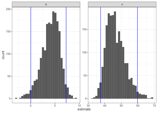
可能なモデル適合度 augment()を使用して、適合曲線の不確実性を視覚化できます。ブートストラップサンプルが多すぎるため、視覚化ではモデル適合度のサンプルのみを表示します。
boot_aug <-
boot_models %>%
sample_n(200) %>%
mutate(augmented = map(model, augment)) %>%
unnest(augmented)
boot_aug
#> # A tibble: 6,400 × 8
#> splits id model coef_info mpg wt .fitted .resid
#> <list> <chr> <list> <list> <dbl> <dbl> <dbl> <dbl>
#> 1 <split [32/11]> Bootstrap1644 <nls> <tibble> 16.4 4.07 15.6 0.829
#> 2 <split [32/11]> Bootstrap1644 <nls> <tibble> 19.7 2.77 21.9 -2.21
#> 3 <split [32/11]> Bootstrap1644 <nls> <tibble> 19.2 3.84 16.4 2.84
#> 4 <split [32/11]> Bootstrap1644 <nls> <tibble> 21.4 2.78 21.8 -0.437
#> 5 <split [32/11]> Bootstrap1644 <nls> <tibble> 26 2.14 27.8 -1.75
#> 6 <split [32/11]> Bootstrap1644 <nls> <tibble> 33.9 1.84 32.0 1.88
#> 7 <split [32/11]> Bootstrap1644 <nls> <tibble> 32.4 2.2 27.0 5.35
#> 8 <split [32/11]> Bootstrap1644 <nls> <tibble> 30.4 1.62 36.1 -5.70
#> 9 <split [32/11]> Bootstrap1644 <nls> <tibble> 21.5 2.46 24.4 -2.86
#> 10 <split [32/11]> Bootstrap1644 <nls> <tibble> 26 2.14 27.8 -1.75
#> # ℹ 6,390 more rowsggplot(boot_aug, aes(wt, mpg)) +
geom_line(aes(y = .fitted, group = id), alpha = .2, col = "blue") +
geom_point()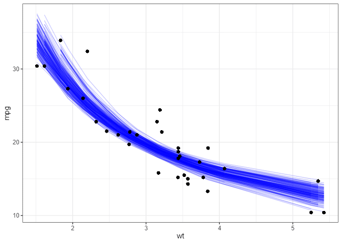
ほんの少しの変更で、tidy()やaugment()関数が多くの統計的な出力に対して機能するため、他の種類の予測や仮説検定モデルでもブートストラップを簡単に実行できます。別の例として、smooth.spline()を使用して、データに対して3次スムージングスプラインを適合させることができます。
fit_spline_on_bootstrap <- function(split) {
data <- analysis(split)
smooth.spline(data$wt, data$mpg, df = 4)
}
boot_splines <-
boots %>%
sample_n(200) %>%
mutate(spline = map(splits, fit_spline_on_bootstrap),
aug_train = map(spline, augment))splines_aug <-
boot_splines %>%
unnest(aug_train)ggplot(splines_aug, aes(x, y)) +
geom_line(aes(y = .fitted, group = id), alpha = 0.2, col = "blue") +
geom_point()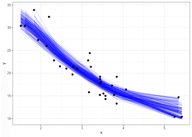
この記事が気に入ったらサポートをしてみませんか?