
ヘボkagglerのTitanic再挑戦【直感失敗編】 #kaggle #機械学習

お世話になっております。
今、Titanicやったらどうなるんだろう??
— ムジンさん:小さなIT会社の社長 (@MKP3share) April 21, 2020
やってみよう。
とんでもない正解率低かったら、細かいことを気にしない私も凹みそうだけれど。
※関係各所へ。機械学習でPCのメモリパンパン=動画制作できんのです。#機械学習 #kaggle
ふと疑問に思ったのでやってみます。
9ヶ月ぶりにタイタニックをやってみることにしました。
ここにいって、
こうする。

new notebookで、START。
データを読み込む
いきなり間違える
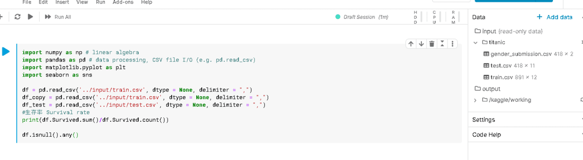
import numpy as np # linear algebra
import pandas as pd # data processing, CSV file I/O (e.g. pd.read_csv)
import matplotlib.pyplot as plt
import seaborn as sns

df = pd.read_csv('../input/train.csv', dtype = None, delimiter = ",")
df_copy = pd.read_csv('../input/train.csv', dtype = None, delimiter = ",")
df_test = pd.read_csv('../input/test.csv', dtype = None, delimiter = ",")
#生存率 Survival rate
print(df.Survived.sum()/df.Survived.count())

df.isnull().any()
titanic抜けてました。一番大事だ。
import numpy as np # linear algebra
import pandas as pd # data processing, CSV file I/O (e.g. pd.read_csv)
import matplotlib.pyplot as plt
import seaborn as sns

df = pd.read_csv('../input/titanic/train.csv', dtype = None, delimiter = ",")
df_copy = pd.read_csv('../input/titanic/train.csv', dtype = None, delimiter = ",")
df_test = pd.read_csv('../input/titanic/test.csv', dtype = None, delimiter = ",")

#生存率 Survival rate
print(df.Survived.sum()/df.Survived.count())

df.isnull().any()df.shape
(891, 12)Survivedの分、カラムが多い。
Survivedをtestの方でも予測して、正解率を上げていこうじゃありませんか。
df_test.shape
(418, 11)
生存率
#生存率 Survival rate
print(df.Survived.sum()/df.Survived.count())
確かTitanicは生き延びたかどうかの判定のはず。
trainで学習、testで予測を。
gender_submission.csvは、送信例だったかな。
女性が全員生存する想定での例、、、だったかな。
生存率を出すのは、私の場合は特に性格が適当なため、適当に判別した時の確率以上に判別できるのが、機械学習の最初の目標となるためです。
※計算合っているか心配だな
欠損値
df.isnull().any()単にnull値、欠損値がある列を見ているだけです。
下に続く行で、カラム名をコピペしやすい。
ペアプロット
sns.pairplot(df)出すだけ出しておく。
多重共線性
df.corr()1なら、要素同士の関係性が深すぎるから消す!消してやるんや!
corr = df.corr()
sns.heatmap(corr, square=True, annot=True)
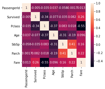
あまり関連性のないカラムは今回は切ってしまおうかと、手抜きを考えてしまうが、、、。
各カラムの型を見る
df.info()
<class 'pandas.core.frame.DataFrame'>
RangeIndex: 891 entries, 0 to 890
Data columns (total 12 columns):
PassengerId 891 non-null int64
Survived 891 non-null int64
Pclass 891 non-null int64
Name 891 non-null object
Sex 891 non-null object
Age 714 non-null float64
SibSp 891 non-null int64
Parch 891 non-null int64
Ticket 891 non-null object
Fare 891 non-null float64
Cabin 204 non-null object
Embarked 889 non-null object
dtypes: float64(2), int64(5), object(5)
memory usage: 83.7+ KBdf_test.info()
<class 'pandas.core.frame.DataFrame'>
RangeIndex: 418 entries, 0 to 417
Data columns (total 11 columns):
PassengerId 418 non-null int64
Pclass 418 non-null int64
Name 418 non-null object
Sex 418 non-null object
Age 332 non-null float64
SibSp 418 non-null int64
Parch 418 non-null int64
Ticket 418 non-null object
Fare 417 non-null float64
Cabin 91 non-null object
Embarked 418 non-null object
dtypes: float64(2), int64(4), object(5)
memory usage: 36.0+ KBobjectっていうのが、だいたい文字列で計算に向かないから、これを機械学習の前に処理します。前に処理します。前処理。
数字にします。
train+testを結合
df = pd.concat([df, df_test])
df.shape
(1309, 12)df.info()
<class 'pandas.core.frame.DataFrame'>
Int64Index: 1309 entries, 0 to 417
Data columns (total 12 columns):
Age            1046 non-null float64
Cabin          295 non-null object
Embarked       1307 non-null object
Fare           1308 non-null float64
Name           1309 non-null object
Parch          1309 non-null int64
PassengerId    1309 non-null int64
Pclass         1309 non-null int64
Sex            1309 non-null object
SibSp          1309 non-null int64
Survived       891 non-null float64
Ticket         1309 non-null object
dtypes: float64(3), int64(4), object(5)
memory usage: 132.9+ KB
改めて欠損値
df.isnull().any()

Age             True
Cabin           True
Embarked        True
Fare            True
Name           False
Parch          False
PassengerId    False
Pclass         False
Sex            False
SibSp          False
Survived        True
Ticket         False
dtype: bool
前処理する前に
for column in df.columns:
   print(column,df[column].unique())
これで各列の数値のユニークな値が、ダラダラ出てくる。
出てきてしまう。だらーっと。こういう雑に全体を見るのがスキ。
Age
数字なのは今までの作業でわかってて、小数点はいらないかと思ってしまった。
df['Age'] = np.round(df.fillna(df['Age'].mean()))欠損値を、全体の平均値で埋めながら、小数点を丸めてしまう。
df['Age'].astype('int8')↑これ、使用メモリ量を浮かすためにやっているんですけど、みなさんどうしているんですかね、、、
Cabin
df['Cabin'] = df['Cabin'].fillna(0)
0埋め。
column = 'Cabin'
labels, uniques = pd.factorize(df[column])
df[column] = labels
print('labels',column)
文字列を数値にラベリング。
Ticket
column = 'Ticket'
labels, uniques = pd.factorize(df[column])
df[column] = labels
print('labels',column)
Sex
column = 'Sex'
df[column] = pd.Categorical(df[column])
df=pd.get_dummies(df,columns=[column],drop_first=True)
性別はダミー変数へ。drop_firstで一列消している。それで表現できるからと知った時は、あーなるほどー頭いい!と思ったものだ。私はこういうのは、言われないと思いつかない脳の持ち主ですから。
Embarked
column = 'Embarked'
df[column] = pd.Categorical(df[column])
df=pd.get_dummies(df,columns=[column],drop_first=True)
同じ。
Name
column = 'Name'
labels, uniques = pd.factorize(df[column])
df[column] = labels
print('labels',column)
初めて見た時に、ファミリーネームで分割したいと思ったのが懐かしい。とりあえず、数値ラベリング。
前処理終わり
機械学習できるところまでとりあえず持っていってしまう。
testデータを抽出
############################################
test_x = df[df['Survived'].isnull()]
test_x = test_x.drop(['Survived'], axis=1)
############################################
Survivedが空のはずなので、その条件で切り出し。
更に予測すべきSurvived列を消す。
機械学習にかけるトレーニング用とトレーニングの正解値を分割
train_y = df['Survived']
train_y = train_y.values
train_y = train_y.astype(np.int8)

train_x = df.drop(['Survived'], axis=1)
train_x = train_x.fillna(0)
カラム名をリストに入れておく
feature_names = list(train_x)
len(feature_names)
12
LightGBMを使う
import lightgbm as lgbデータを学習しやすい形に更に分割
from sklearn.model_selection import train_test_split
tr_x, va_x, tr_y, va_y = train_test_split(train_x, train_y,random_state=None, shuffle=False)
ランダムに分割しない。シャッフルもしないで、トレーニング用データを更に分割。トレーニング中にva_xを使って予習復習みたいなことをしてもらいます。
1回目の学習
best_params = {
   'objective': 'binary',
   'metric': 'auc',
   'save_binary': True,
   'verbose': 1,
   'n_estimators': 50000,
   'boosting': 'gbdt',
}
############################################
from sklearn.metrics import accuracy_score, recall_score, precision_score, f1_score

trn_data = lgb.Dataset(train_x, label=train_y, feature_name=feature_names)
val_data = lgb.Dataset(va_x, label=va_y, reference=trn_data)

model = lgb.train(best_params, trn_data, num_boost_round = 1000, valid_sets = [trn_data, val_data],early_stopping_rounds=50)
Early stopping, best iteration is:
[1] training's auc: 0.914422 valid_1's auc: 1ふむ?
1回目の結果
predict = model.predict(test_x, num_iteration=model.best_iteration)
y_pred_max = np.round(predict)
print(predict)
print(y_pred_max)
0.3146185 0.31705838 0.3146185 0.3146185 0.3146185 0.35865407
0.33391247 0.31705838 0.3146185 0.3146185 0.3146185 0.31705838
0.3146185 0.31705838 0.3146185 0.3146185 0.31705838 0.3146185
0.31705838 0.3146185 0.33391247 0.33391247 0.3146185 0.32419081
0.31705838 0.31705838 0.31705838 0.31705838 0.31705838 0.3146185
あら?分類できてない。全部0になっちゃうぞ。
データ分割からやり直し
from sklearn.model_selection import train_test_split
train_x, va_x, train_y, va_y = train_test_split(train_x, train_y,random_state=42, shuffle=True)
これでも変。
 0.0066175  0.00504281 0.00559275 0.00504281 0.00504281 0.00734264
0.00504281 0.00504281 0.00504281 0.00504281 0.00504281 0.00504281
0.00504281 0.00559429 0.0066175  0.0066175  0.00504281 0.0066175
0.00504281 0.00504079 0.00504281 0.00504281 0.00504281 0.00504281
なんだっけな?
各カラムの重要度を出力
# 特徴量の重要度をプロットする
lgb.plot_importance(clf, figsize=(20, 20))
plt.show()
チケット?なんか変だな。チケットを適当にラベリングした奴がいちばん重要だと??
プログラムの見直し
df_result_dropna = df.dropna(subset=['Survived'])
feature_names = df_result_dropna.drop(['Survived'], axis=1)

train_y = df_result_dropna['Survived']
train_x = df_result_dropna.drop(['Survived'], axis=1)
#train_x = train_x.values
すぐ見つかりました。
テスト用のデータ分を切り落とし忘れていました。
test_x = test_x.values
train_x = train_x.values
値をnumpy配列にして機械学習します。
train_x.dtypes

AttributeError: 'numpy.ndarray' object has no attribute 'dtypes'
機械学習を実行し、小数点丸め
predict = model.predict(test_x, num_iteration=model.best_iteration)
y_pred_max = np.round(predict)
print(predict)
print(y_pred_max)
特徴量の重要度
# 特徴量の重要度をプロットする
lgb.plot_importance(model, figsize=(20, 20))
plt.show()
ふむふむ。ふむ?
出力用ファイルを作成
df_test['PassengerId']
df_sub提出例のファイルとテストデータのIDが一緒みたいなので、そこにそのまま結果を突っ込む。
df_sub['Survived'] = y_pred_max
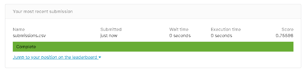
正解率:75%
なんにも考えないで75%。
Fare
column = 'Fare'
df[column] = np.round(df.fillna(df[column].mean()))
print('labels',column)
運賃の数値が細かすぎるので、ちょいと丸める。
正解率:77.9%(0.77990)

細かい数字をまとめると、正解率が向上した。
グループ分けのように、数値ごとにグループ分けしてみよう。
Ageの99パーセンタイル
df['Age'] = np.round(df.fillna(df['Age'].mean()))
df['Age'].astype('int8')
df['Age'].unique()

column = 'Age'
upperbound, lowerbound = np.percentile(df[column], [1, 99])
Age = np.clip(df[column], upperbound, lowerbound)
print(Age.unique)
小さい順に並べて、どの辺りにその値があるかで、分割するっていうかなんていうか。
numpyにするところをStandardScaler
from sklearn.preprocessing import StandardScaler
ss = StandardScaler()
train_x = ss.fit_transform(train_x)
test_x = ss.fit_transform(test_x)
意味ないかもな。もうクセみたいになっているけれど。
これで、正解率はいかほどか?

あら?終わらない。待つのもなんなので先に行こう。
NameとCabinの分割
mr missとかは名前から切り出すのが楽だから、それを実行。
同じパターンでCavinの数字とアルファベットを分割。
意味あるなしに関わらず、やれることは全部やる方式なので、文字列の意味などは考えていません。
機械的に処理を遂行しています。
正規表現チェッカーで何度もテストして、思った文字列が出るまで試します。
df['CabinHead'] = df[column].str.extract('([A-Za-z]+)', expand = False)df['mrms'] = df['Name'].str.extract('([A-Za-z]+)\.', expand = False)
df['mrms'].unique()
array(['Mr', 'Mrs', 'Miss', 'Master', 'Don', 'Rev', 'Dr', 'Mme', 'Ms',
'Major', 'Lady', 'Sir', 'Mlle', 'Col', 'Capt', 'Countess',
'Jonkheer', 'Dona'], dtype=object)正規表現、苦手だなー。
途中の正解率

78.4%
ちょっと向上。
多重共線性

あ!1があるな。消さないといかん。
いらなそうなカラムを消す
PassengerIdは学習時は落とそう。
mrms_Donaが邪魔だな。
むぅ、、、
問題はTicket。
意味ないはずが、重要度が高いと出ている。
消してみるか。
Ticketを消した正解率

78.9%
ちょっと向上。
遺伝的プログラミング
pip install tpotfrom tpot import TPOTClassifier
tpot = TPOTClassifier(generations=5, population_size=20, verbosity=2)
tpot.fit(train_x, train_y)
print(tpot.score(train_x, train_y))こいつに特徴量の謎を解かずに、無理やりベストなアルゴリズムやらなんやらを出させる。腕力だ!
Generation 1 - Current best internal CV score: 0.8305316678174629
Generation 2 - Current best internal CV score: 0.8316427091833531
Generation 3 - Current best internal CV score: 0.8316427091833531
Generation 4 - Current best internal CV score: 0.8316427091833531
Generation 5 - Current best internal CV score: 0.8327725817588348
Best pipeline: ExtraTreesClassifier(input_matrix, bootstrap=True, criterion=entropy, max_features=0.8, min_samples_leaf=5, min_samples_split=14, n_estimators=100)
0.8608305274971941
ほー。
ExtraTreesClassifierの実装

ぬぅ。下がった。
いや、適当に書いたから、実装の仕方を間違えている部分もある。
特徴量の見直し
まだデータの性質は見ないぞ!
indexの数値がおかしいので、
df.reset_index(drop=True,inplace=True)を
df = pd.concat([df, df_test])の下辺りに追加。
特徴量の自動生成
df_y = df['Survived']
df_x = df.drop(['PassengerId','Survived'], axis=1)

import featuretools as ft

# Entity Setの作成
es = ft.EntitySet(id='entityset')

# Entityの追加
es = es.entity_from_dataframe(entity_id='train',dataframe=df_x,index='index')

# 特徴量の生成
feature_matrix, features_defs = ft.dfs(
   entityset=es,
   target_entity="train",
   agg_primitives=["count","mean", "max", "min", "std", "skew"],
   trans_primitives=['cum_max','and','not','diff'],
   max_depth=3
   )

# 特徴量の確認
feature_matrix.info()
print(feature_matrix.shape)
df = feature_matrix

df['Survived'] = df_y
Survivedを一旦退避しておいて、数値列を適当に組み合わせて、特徴量を増加させます。
1309 rows × 93 columnsいらない特徴量を消す

白いところを地道に消す。
df = df.drop(['CUM_MAX(Sex_male)','CUM_MAX(mrms_Mr)','CUM_MAX(Pclass)','CUM_MAX(Embarked_S)'], axis=1)
df = df.drop(['DIFF(CUM_MAX(Pclass))','DIFF(CUM_MAX(Embarked_S))','DIFF(CUM_MAX(mrms_Mr))','DIFF(CUM_MAX(Sex_male))','CUM_MAX(CabinHead_C)','CUM_MAX(mrms_Mrs)'], axis=1)
まだ多重共線性があるが、一度全体を動かしてみよう。
っと、
0埋め
特徴量を増加させたが、
train_x=train_x.fillna(0)
test_x=test_x.fillna(0)
然るべきところで、0埋めしておこう。
再度、機械学習
ここまで雑に進行できる所に、精度の低さの危機感よりも、成長を先に感じてしまう、、、
これでバージョン16です。
※このタイミングで、競輪のデータ生成第一弾がやっと終わった。
既に何度も結果のSubmitを行ってしまったので、後日改めて結果を確認しよう。
・・・
下がってるやん。
反省して、しっかりデータを見よう。
df_train
df_train = pd.read_csv('../input/titanic/train.csv', dtype = None, delimiter = ",")最初から気になっていたので変更。
元データが存在し続ける方が、途中で処理データと元データと比較できていい。
Ageの再処理
df['Age'].value_counts()0.67、、、やはりroundでの丸めは実施しよう。
df['Age'] = np.round(df.fillna(df['Age'].mean()))山なりに綺麗にデータを並べてみよう

sns.catplot(x='Age', col='Survived', kind='count', data=df_train,height=10, aspect=2)train+testのAgeのbin分割
ええとこで区切ります。※qcutでない
df['Age'] = np.round(df.fillna(df['Age'].mean()))

column = 'Age'
df[column+'bin'] = pd.cut(df[column], 6, labels=False, precision=1)

sns.catplot(x='Agebin', col='Survived', kind='count', data=df,height=10, aspect=2);

5分割でいいか。
正規分布の感じを出さないとダメなんやろな。
以下は一応。
print(df['Age'].unique)

column = 'Age'
upperbound, lowerbound = np.percentile(df[column], [1, 99])
df['Age'] = np.clip(df[column], upperbound, lowerbound)

print(df['Age'].unique)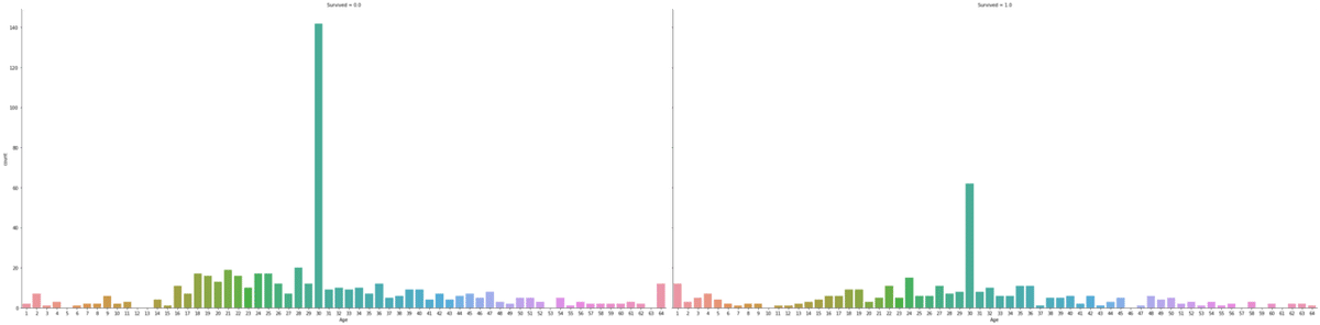
偏り!
これで、重要度を見てみると、AgeとAgebinが0.9で相関が高いので、Ageを切る。
Agebinの可視化
plt.hist(df['Agebin'], bins=4)
df['Agebin'].unique()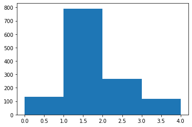
g = sns.FacetGrid(df, col='Survived')
g.map(plt.hist, 'Agebin', bins=5)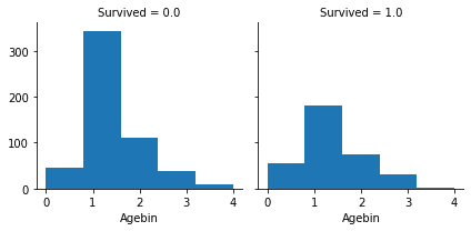
うーむ。
Ticketの再処理
df['Ticket'].value_counts()

CA. 2343    7
347082      7
1601        7
3101295     6
CA 2144     6
          ..
PC 17476    1
350417      1
11753       1
PP 4348     1
334912      1
Name: Ticket, Length: 681, dtype: int64
column = 'Ticket'
labels, uniques = pd.factorize(df[column])
df[column] = labels
print('labels',column)df['Ticket'].value_counts()Fareの再処理:ミスに気付く
df[column].isnull().any()
Truedf[column].isnull().sum()
1df[column].value_counts()
8.0500 60
13.0000 59
7.7500 55
26.0000 50
7.8958 49
..
8.0292 1
12.7375 1
8.6542 1
34.0208 1
7.1417 1
Name: Fare, Length: 282, dtype: int64ミスの修正
df[column] = np.round(df.fillna(df[column].mean()))
df[column] = df[column].fillna(df[column].mean())全体のNaNをFareの平均で埋めてしまっていたが、これでFareのみになった。
Nameの謎
何故か名前に重要度があるように出力される。
法則性も見えないし、重複する同姓同名で生存した人が多いわけでもない。
???
消すか。
featuretools
name	type	description
0	avg_time_between	aggregation	Computes
the average number
o

f seconds between...
1	time_since_last	aggregation	Calculates the time elapsed since the last dat...
2	min	aggregation	Calculates the smallest value, ignoring `NaN` ...
3	time_since_first	aggregation	Calculates the time elapsed since the first da...
4	any	aggregation	Determines if any value is 'True' in a list.
5	entropy	aggregation	Calculates the entropy for a categorical variable
6	mean	aggregation	Computes the average for a list of values.
7	n_most_common	aggregation	Determines the `n` most common elements.
8	trend	aggregation	Calculates the trend of a variable over time.
9	first	aggregation	Determines the first value in a list.
10	num_true	aggregation	Counts the number of `True` values.
11	skew	aggregation	Computes the extent to which a distribution di...
12	count	aggregation	Determines the total number of values, excludi...
13	max	aggregation	Calculates the highest value, ignoring `NaN` v...
14	all	aggregation	Calculates if all values are 'True' in a list.
15	mode	aggregation	Determines the most commonly repeated value.
16	last	aggregation	Determines the last value in a list.
17	sum	aggregation	Calculates the total addition, ignoring `NaN`.
18	percent_true	aggregation	Determines the percent of `True` values.
19	std	aggregation	Computes the dispersion relative to the mean v...
20	num_unique	aggregation	Determines the number of distinct values, igno...
21	median	aggregation	Determines the middlemost number in a list of ...
22	equal	transform	Determines if values in one list are equal to ...
23	week	transform	Determines the week of the year from a datetime.
24	greater_than	transform	Determines if values in one list are greater t...
25	is_weekend	transform	Determines if a date falls on a weekend.
26	modulo_numeric	transform	Element-wise modulo of two lists.
27	less_than_scalar	transform	Determines if values are less than a given sca...
28	less_than_equal_to	transform	Determines if values in one list are less than...
29	percentile	transform	Determines the percentile rank for each value ...
30	second	transform	Determines the seconds value of a datetime.
31	negate	transform	Negates a numeric value.
32	time_since	transform	Calculates time from a value to a specified cu...
33	day	transform	Determines the day of the month from a datetime.
34	cum_mean	transform	Calculates the cumulative mean.
35	isin	transform	Determines whether a value is present in a pro...
36	num_characters	transform	Calculates the number of characters in a string.
37	year	transform	Determines the year value of a datetime.
38	absolute	transform	Computes the absolute value of a number.
39	time_since_previous	transform	Compute the time since the previous entry in a...
40	cum_sum	transform	Calculates the cumulative sum.
41	add_numeric_scalar	transform	Add a scalar to each value in the list.
42	cum_max	transform	Calculates the cumulative maximum.
43	multiply_boolean	transform	Element-wise multiplication of two lists of bo...
44	not_equal_scalar	transform	Determines if values in a list are not equal t...
45	greater_than_equal_to_scalar	transform	Determines if values are greater than or equal...
46	haversine	transform	Calculates the approximate haversine distance ...
47	and	transform	Element-wise logical AND of two lists.
48	multiply_numeric	transform	Element-wise multiplication of two lists.
49	equal_scalar	transform	Determines if values in a list are equal to a ...
50	greater_than_scalar	transform	Determines if values are greater than a given ...
51	latitude	transform	Returns the first tuple value in a list of Lat...
52	modulo_numeric_scalar	transform	Return the modulo of each element in the list ...
53	or	transform	Element-wise logical OR of two lists.
54	less_than_equal_to_scalar	transform	Determines if values are less than or equal to...
55	scalar_subtract_numeric_feature	transform	Subtract each value in the list from a given s...
56	minute	transform	Determines the minutes value of a datetime.
57	subtract_numeric_scalar	transform	Subtract a scalar from each element in the list.
58	divide_numeric_scalar	transform	Divide each element in the list by a scalar.
59	divide_by_feature	transform	Divide a scalar by each value in the list.
60	less_than	transform	Determines if values in one list are less than...
61	not	transform	Negates a boolean value.
62	hour	transform	Determines the hour value of a datetime.
63	diff	transform	Compute the difference between the value in a ...
64	num_words	transform	Determines the number of words in a string by ...
65	cum_count	transform	Calculates the cumulative count.
66	month	transform	Determines the month value of a datetime.
67	weekday	transform	Determines the day of the week from a datetime.
68	subtract_numeric	transform	Element-wise subtraction of two lists.
69	is_null	transform	Determines if a value is null.
70	divide_numeric	transform	Element-wise division of two lists.
71	add_numeric	transform	Element-wise addition of two lists.
72	cum_min	transform	Calculates the cumulative minimum.
73	multiply_numeric_scalar	transform	Multiply each element in the list by a scalar.
74	not_equal	transform	Determines if values in one list are not equal...
75	greater_than_equal_to	transform	Determines if values in one list are greater t...
76	longitude	transform	Returns the second tuple value in a list of La...
77	modulo_by_feature	transform	Return the modulo of a scalar by each element ...
適当に貼っていたfeaturetoolsをしっかり動かす。
# Entity Setの作成
es = ft.EntitySet(id='entityset')
# Entityの追加
# 親テーブル
es = es.entity_from_dataframe(entity_id='train',dataframe=df_x,index='index')
# 特徴量の生成
feature_matrix, features_defs = ft.dfs(
   entityset=es,
   target_entity='train',
   agg_primitives=['max'],
   trans_primitives=['add_numeric','subtract_numeric','multiply_numeric','divide_numeric','cum_max','diff'],
   max_depth=1
   )
# 特徴量の確認
feature_matrix.info()
print(feature_matrix.shape)
dfs = feature_matrix
とりあえずこんな感じで四則演算メイン。
1309 rows × 1010 columnsになる。
これだと特徴量を絞り込む必要が出る。
特徴量の絞り込み
from sklearn.feature_selection import SelectKBest
from sklearn.feature_selection import f_classif
selector = SelectKBest(f_classif, k=100)
selector.fit(train_x,train_y)
この辺、適当ですが、だいたいドキュメントどおりにやっています。
mask = selector.get_support() #list of booleans
new_features = [] # The list of your K best features
for bool, feature in zip(mask, feature_names):
   if bool:
       new_features.append(feature)
選択した特徴量を見る。どこかの質問の回答から引用。
X_train_selected = selector.transform(train_x)
X_test_selected = selector.transform(test_x)
これで直感でのモデルはほぼ完成かな。これの改良で80%超えなかったら悲しいな。
結果
78.9%😫
と
76%
全然ダメやないか。
やはり、ここまできて基本に立ち返るのが大事なんだろうな。
9ヶ月前の自分の成績を超えないっていうのも問題だ。
一旦、Titanicをやり直してみよう。
kaggle kernel
いつもお読みいただき、ありがとうございます。 書くだけでなく読みたいので、コメント欄で記事名入れてもらうと見に行きます。