
第12章:戦略をブースティングする 第1節: ブースティング・ベースライン

はじめに
とうとう第12章です。ここで教師あり学習は終わって、13章以降は深層学習含めた教師なし学習をメインに取り扱います。また、教師あり学習のケースでも深層学習を取り扱ったりします。
※以下は個人的な見解になります。
この章まで出来れば機械学習及びファクター投資の知識としてはほぼ十分かと思われます。
実際、深層学習を用いたトレーディング手法はかなり研究されておりますが、難易度も高く、投資においてはブラックボックスになること自体がリスクであるので、実務上で使われるためにはかなりのハードルをクリアする必要があります。
それと比べて、ファクター投資とアンサンブルモデルによる学習は、負けた時にファクターがこの場面では効かなかった等、言い訳がつけやすく、モデルの向上もさせやすいため、難易度はどちらも高いですが、扱いやすさは断然ファクター研究の方になります。
インポートと設定
%matplotlib inline

import sys, os
import warnings
from time import time
from itertools import product
import joblib
from pathlib import Path
import numpy as np
import pandas as pd

import matplotlib.pyplot as plt
from matplotlib.ticker import FuncFormatter
from mpl_toolkits.mplot3d import Axes3D
import seaborn as sns

from xgboost import XGBClassifier
from lightgbm import LGBMClassifier
from catboost import CatBoostClassifier
from sklearn.model_selection import cross_validate
from sklearn.dummy import DummyClassifier
from sklearn.tree import DecisionTreeClassifier
from sklearn.ensemble import RandomForestClassifier, AdaBoostClassifier, GradientBoostingClassifier
from sklearn.inspection import partial_dependence, plot_partial_dependence
from sklearn.metrics import roc_auc_scoresys.path.insert(1, os.path.join(sys.path[0], '..'))
from utils import format_timeresults_path = Path('results', 'baseline')
if not results_path.exists():
results_path.mkdir(exist_ok=True, parents=True)warnings.filterwarnings('ignore')
sns.set_style("whitegrid")
idx = pd.IndexSlice
np.random.seed(42)データの準備
4章アルファ-ファクター研究: 第一節: 特徴量エンジニアリングからデータを作成してください。
DATA_STORE = '../data/assets.h5'def get_data(start='2000', end='2018', task='classification', holding_period=1, dropna=False):
idx = pd.IndexSlice
target = f'target_{holding_period}m'
with pd.HDFStore(DATA_STORE) as store:
df = store['engineered_features']
if start is not None and end is not None:
df = df.loc[idx[:, start: end], :]
if dropna:
df = df.dropna()
y = (df[target]>0).astype(int)
X = df.drop([c for c in df.columns if c.startswith('target')], axis=1)
return y, Xカテゴリーに分解する
cat_cols = ['year', 'month', 'age', 'msize', 'sector']def factorize_cats(df, cats=['sector']):
cat_cols = ['year', 'month', 'age', 'msize'] + cats
for cat in cats:
df[cat] = pd.factorize(df[cat])[0]
df.loc[:, cat_cols] = df.loc[:, cat_cols].fillna(-1).astype(int)
return dfONE-HOT エンコーディング
One-hotに関してはこちら
以下引用
デジタル回路において、one-hot(ワン・ホット)は1つだけHigh(1)であり、他はLow(0)であるようなビット列のことを指す。 類似のものとして、0が1つだけで、他がすべて1であるようなビット列をone-cold(ワン・コールド)と呼ぶことがある。
def get_one_hot_data(df, cols=cat_cols[:-1]):
   df = pd.get_dummies(df,
                       columns=cols + ['sector'],
                       prefix=cols + [''],
                       prefix_sep=['_'] * len(cols) + [''])
   return df.rename(columns={c: c.replace('.0', '') for c in df.columns})
ホールドアウト法
ホールドアウト法に関しては、こちら
以下引用です。
教師あり学習を行う上で、モデルを作成し評価するための基本的な手法
教師ありデータを学習データとテストデータに分割する。
学習データでモデルを作成し、テストデータで性能を図る。
より効果的な方法として、データを学習データ、検証データ、テストデータと3つに分割し、検証データによって複数のモデルを評価・選択して最終的にテストデータで汎化誤差を評価する方法がある。
よく取られる手法です。
def get_holdout_set(target, features, period=6):
   idx = pd.IndexSlice
   label = target.name
   dates = np.sort(y.index.get_level_values('date').unique())
   cv_start, cv_end = dates[0], dates[-period - 2]
   holdout_start, holdout_end = dates[-period - 1], dates[-1]

   df = features.join(target.to_frame())
   train = df.loc[idx[:, cv_start: cv_end], :]
   y_train, X_train = train[label], train.drop(label, axis=1)

   test = df.loc[idx[:, holdout_start: holdout_end], :]
   y_test, X_test = test[label], test.drop(label, axis=1)
   return y_train, X_train, y_test, X_test
データの読み込み
y, features = get_data()
X_dummies = get_one_hot_data(features)
X_factors = factorize_cats(features)
X_factors.info()
'''
<class 'pandas.core.frame.DataFrame'>
MultiIndex: 358914 entries, ('A', Timestamp('2001-01-31 00:00:00')) to ('ZUMZ', Timestamp('2018-02-28 00:00:00'))
Data columns (total 27 columns):
# Column Non-Null Count Dtype
--- ------ -------------- -----
0 return_1m 358914 non-null float64
1 return_2m 358914 non-null float64
2 return_3m 358914 non-null float64
3 return_6m 358914 non-null float64
4 return_9m 358914 non-null float64
5 return_12m 358914 non-null float64
6 Mkt-RF 358914 non-null float64
7 SMB 358914 non-null float64
8 HML 358914 non-null float64
9 RMW 358914 non-null float64
10 CMA 358914 non-null float64
11 momentum_2 358914 non-null float64
12 momentum_3 358914 non-null float64
13 momentum_6 358914 non-null float64
14 momentum_9 358914 non-null float64
15 momentum_12 358914 non-null float64
16 year 358914 non-null int64
17 month 358914 non-null int64
18 return_1m_t-1 357076 non-null float64
19 return_1m_t-2 355238 non-null float64
20 return_1m_t-3 353400 non-null float64
21 return_1m_t-4 351562 non-null float64
22 return_1m_t-5 349724 non-null float64
23 return_1m_t-6 347886 non-null float64
24 age 358914 non-null int64
25 msize 358914 non-null int64
26 sector 358914 non-null int64
dtypes: float64(22), int64(5)
memory usage: 85.3+ MB
'''y_clean, features_clean = get_data(dropna=True)
X_dummies_clean = get_one_hot_data(features_clean)
X_factors_clean = factorize_cats(features_clean)交差検証セットアップ
カスタム時系列Kフォールド生成器
class OneStepTimeSeriesSplit:
   """Generates tuples of train_idx, test_idx pairs
   Assumes the index contains a level labeled 'date'"""

   def __init__(self, n_splits=3, test_period_length=1, shuffle=False):
       self.n_splits = n_splits
       self.test_period_length = test_period_length
       self.shuffle = shuffle

   @staticmethod
   def chunks(l, n):
       for i in range(0, len(l), n):
           yield l[i:i + n]

   def split(self, X, y=None, groups=None):
       unique_dates = (X.index
                       .get_level_values('date')
                       .unique()
                       .sort_values(ascending=False)
                       [:self.n_splits*self.test_period_length])

       dates = X.reset_index()[['date']]
       for test_date in self.chunks(unique_dates, self.test_period_length):
           train_idx = dates[dates.date < min(test_date)].index
           test_idx = dates[dates.date.isin(test_date)].index
           if self.shuffle:
               np.random.shuffle(list(train_idx))
           yield train_idx, test_idx

   def get_n_splits(self, X, y, groups=None):
       return self.n_splits
cv = OneStepTimeSeriesSplit(n_splits=12,
test_period_length=1,
shuffle=False)run_time = {}CV 評価関数
metrics = {'balanced_accuracy': 'Accuracy' ,
          'roc_auc': 'AUC',
          'neg_log_loss': 'Log Loss',
          'f1_weighted': 'F1',
          'precision_weighted': 'Precision',
          'recall_weighted': 'Recall'
}
def run_cv(clf, X=X_dummies, y=y, metrics=metrics, cv=cv, fit_params=None, n_jobs=-1):
start = time()
scores = cross_validate(estimator=clf,
X=X,
y=y,
scoring=list(metrics.keys()),
cv=cv,
return_train_score=True,
n_jobs=n_jobs,
verbose=1,
fit_params=fit_params)
duration = time() - start
return scores, durationCV結果ハンドラー関数
CVの結果を操作してプロットする補助関数
def stack_results(scores):
   columns = pd.MultiIndex.from_tuples(
       [tuple(m.split('_', 1)) for m in scores.keys()],
       names=['Dataset', 'Metric'])
   data = np.array(list(scores.values())).T
   df = (pd.DataFrame(data=data,
                      columns=columns)
         .iloc[:, 2:])
   results = pd.melt(df, value_name='Value')
   results.Metric = results.Metric.apply(lambda x: metrics.get(x))
   results.Dataset = results.Dataset.str.capitalize()
   return results
def plot_result(df, model=None, fname=None):
m = list(metrics.values())
g = sns.catplot(x='Dataset',
y='Value',
hue='Dataset',
col='Metric',
data=df,
col_order=m,
order=['Train', 'Test'],
kind="box",
col_wrap=3,
sharey=False,
height=4, aspect=1.2)
df = df.groupby(['Metric', 'Dataset']).Value.mean().unstack().loc[m]
for i, ax in enumerate(g.axes.flat):
s = f"Train: {df.loc[m[i], 'Train']:>7.4f}\nTest: {df.loc[m[i], 'Test'] :>7.4f}"
ax.text(0.05, 0.85, s, fontsize=10, transform=ax.transAxes,
bbox=dict(facecolor='white', edgecolor='grey', boxstyle='round,pad=0.5'))
g.fig.suptitle(model, fontsize=16)
g.fig.subplots_adjust(top=.9)
if fname:
g.savefig(fname, dpi=300);ベースライン分類器
dummy_clf = DummyClassifier(strategy='stratified',
                           random_state=42)
algo = 'dummy_clf'fname = results_path / f'{algo}.joblib'
if not Path(fname).exists():
dummy_cv_result, run_time[algo] = run_cv(dummy_clf)
joblib.dump(dummy_cv_result, fname)
else:
dummy_cv_result = joblib.load(fname)dummy_result = stack_results(dummy_cv_result)
dummy_result.groupby(['Metric', 'Dataset']).Value.mean().unstack()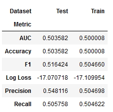
plot_result(dummy_result, model='Dummy Classifier')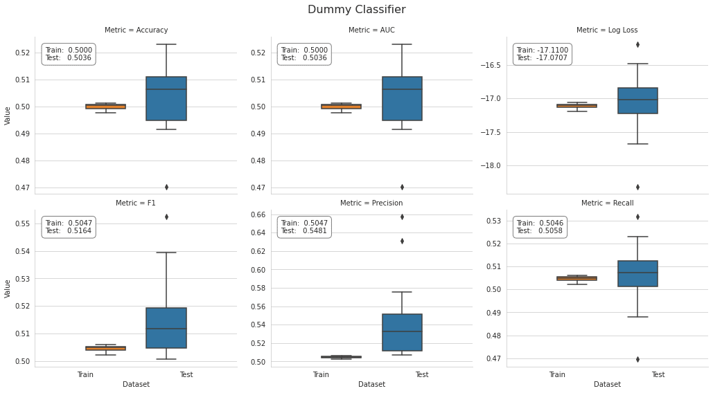
ランダムフォレスト
設定
rf_clf = RandomForestClassifier(n_estimators=100,
                               criterion='gini',
                               max_depth=None,
                               min_samples_split=2,
                               min_samples_leaf=1,
                               min_weight_fraction_leaf=0.0,
                               max_features='auto',
                               max_leaf_nodes=None,
                               min_impurity_decrease=0.0,
                               min_impurity_split=None,
                               bootstrap=True,
                               oob_score=True,
                               n_jobs=-1,
                               random_state=42,
                               verbose=1)
交差検証
algo = 'random_forest'fname = results_path / f'{algo}.joblib'
if not Path(fname).exists():
rf_cv_result, run_time[algo] = run_cv(rf_clf, y=y_clean, X=X_dummies_clean)
joblib.dump(rf_cv_result, fname)
else:
rf_cv_result = joblib.load(fname)結果のプロット
rf_result = stack_results(rf_cv_result)
rf_result.groupby(['Metric', 'Dataset']).Value.mean().unstack()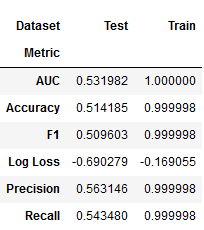
plot_result(rf_result, model='Random Forest')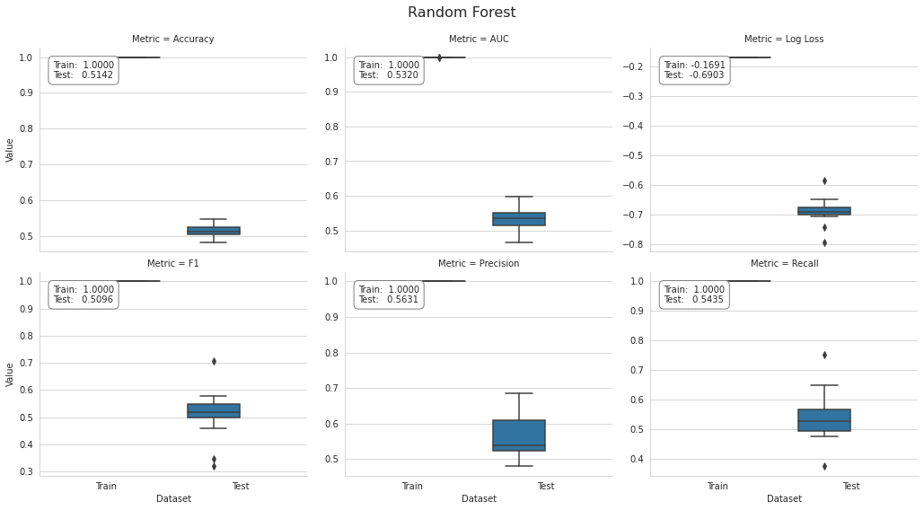
AdaBoost
前の章で説明したように、max_depthへの変更は、min_samples_splitなどの調整を使用して、適切な正則化制約と組み合わせる必要があります。
base_estimator = DecisionTreeClassifier(criterion='gini',
                                       splitter='best',
                                       max_depth=1,
                                       min_samples_split=2,
                                       min_samples_leaf=20,
                                       min_weight_fraction_leaf=0.0,
                                       max_features=None,
                                       random_state=None,
                                       max_leaf_nodes=None,
                                       min_impurity_decrease=0.0,
                                       min_impurity_split=None,
                                       class_weight=None)
設定
ada_clf = AdaBoostClassifier(base_estimator=base_estimator,
                            n_estimators=100,
                            learning_rate=1.0,
                            algorithm='SAMME.R',
                            random_state=42)
交差検証
algo = 'adaboost'fname = results_path / f'{algo}.joblib'
if not Path(fname).exists():
ada_cv_result, run_time[algo] = run_cv(ada_clf, y=y_clean, X=X_dummies_clean)
joblib.dump(ada_cv_result, fname)
else:
ada_cv_result = joblib.load(fname)結果のプロット
ada_result = stack_results(ada_cv_result)
ada_result.groupby(['Metric', 'Dataset']).Value.mean().unstack()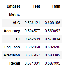
plot_result(ada_result, model='AdaBoost')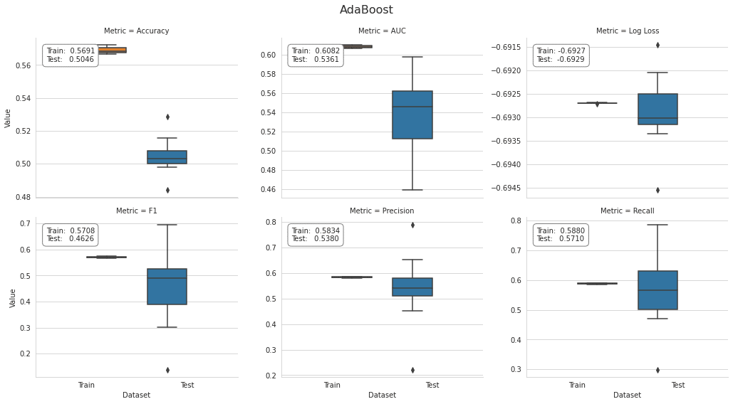
GradientBoostingClassifier
設定
gb_clf = GradientBoostingClassifier(loss='deviance',                # deviance = logistic reg; exponential: AdaBoost
                                   learning_rate=0.1,              # shrinks the contribution of each tree
                                   n_estimators=100,               # number of boosting stages
                                   subsample=1.0,                  # fraction of samples used t fit base learners
                                   criterion='friedman_mse',       # measures the quality of a split
                                   min_samples_split=2,
                                   min_samples_leaf=1,
                                   min_weight_fraction_leaf=0.0,   # min. fraction of sum of weights
                                   max_depth=3,                    # opt value depends on interaction
                                   min_impurity_decrease=0.0,
                                   min_impurity_split=None,
                                   init=None,
                                   random_state=None,
                                   max_features=None,
                                   verbose=0,
                                   max_leaf_nodes=None,
                                   warm_start=False,
                                   presort='auto',
                                   validation_fraction=0.1,
                                   n_iter_no_change=None,
                                   tol=0.0001)
交差検証
algo = 'sklearn_gbm'fname = results_path / f'{algo}.joblib'
if not Path(fname).exists():
gb_cv_result, run_time[algo] = run_cv(gb_clf, y=y_clean, X=X_dummies_clean)
joblib.dump(gb_cv_result, fname)
else:
gb_cv_result = joblib.load(fname)結果のプロット
gb_result = stack_results(gb_cv_result)
gb_result.groupby(['Metric', 'Dataset']).Value.mean().unstack()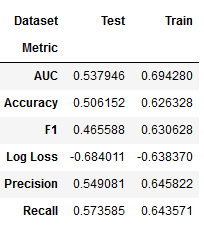
plot_result(gb_result, model='Gradient Boosting Classifier')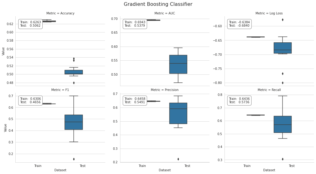
Partial Dependence Plot
こちらの記事参考。
以下引用です。
各変数の重要度がわかったら、次に行うべきは重要な変数とアウトカムの関係を見ることだと思います。 ただ、一般にブラックボックスモデルにおいてインプットとアウトカムの関係は非常に複雑で、可視化することは困難です。
そこで、複雑な関係を要約する手法の一つにPartial Dependence Plot(PDP)があります。PDPは興味のある変数以外の影響を周辺化して消してしまうことで、インプットとアウトカムの関係を単純化しようというものです。
X_ = X_factors_clean.drop(['year', 'month'], axis=1)fname = results_path / f'{algo}_model.joblib'
if not Path(fname).exists():
gb_clf.fit(y=y_clean, X=X_)
joblib.dump(gb_clf, fname)
else:
gb_clf = joblib.load(fname)# mean accuracy
gb_clf.score(X=X_, y=y_clean)
'''
0.5611655700281992
'''y_score = gb_clf.predict_proba(X_)[:, 1]
roc_auc_score(y_score=y_score, y_true=y_clean)
'''
0.5640006909636653
'''特徴量重要度
(pd.Series(gb_clf.feature_importances_,
         index=X_.columns)
.sort_values(ascending=False)
.head(15)).sort_values().plot.barh(title='Feature Importance')
sns.despine()
plt.tight_layout();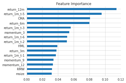
One-wayとTwo-way PDP
fig, axes = plt.subplots(nrows=2, ncols=2, figsize=(12, 10))

plot_partial_dependence(
   estimator=gb_clf,
   X=X_,
   features=['return_12m', 'return_6m', 'CMA', ('return_12m', 'return_6m')],
   percentiles=(0.05, 0.95),
   n_jobs=-1,
   n_cols=2,
   response_method='decision_function',
   grid_resolution=250,
   ax=axes)

for i, j in product([0, 1], repeat=2):
   if i!=1 or j!= 0:
       axes[i][j].xaxis.set_major_formatter(FuncFormatter(lambda y, _: '{:.0%}'.format(y)))

axes[1][1].yaxis.set_major_formatter(FuncFormatter(lambda y, _: '{:.0%}'.format(y)))

axes[0][0].set_ylabel('Partial Dependence')
axes[1][0].set_ylabel('Partial Dependence')
axes[0][0].set_xlabel('12-Months Return')
axes[0][1].set_xlabel('6-Months Return')
axes[1][0].set_xlabel('Conservative Minus Aggressive')

axes[1][1].set_xlabel('12-Month Return')
axes[1][1].set_ylabel('6-Months Return')
fig.suptitle('Partial Dependence Plots', fontsize=16)
fig.tight_layout()
fig.subplots_adjust(top=.95)
fig.savefig('figures/partial_dep_2d', dpi=300);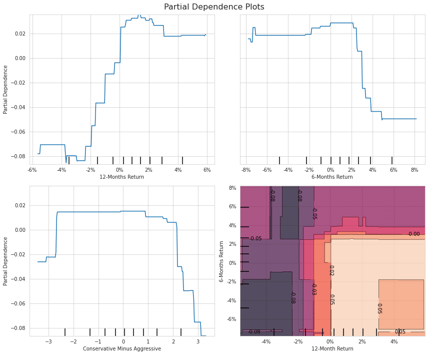
Two-way partial dependence 3D plot
targets = ['return_12m', 'return_6m']
pdp, axes = partial_dependence(estimator=gb_clf,
                              features=targets,
                              X=X_,
                              grid_resolution=100)

XX, YY = np.meshgrid(axes[0], axes[1])
Z = pdp[0].reshape(list(map(np.size, axes))).T

fig = plt.figure(figsize=(14, 8))
ax = Axes3D(fig)
surface = ax.plot_surface(XX, YY, Z,
                         rstride=1,
                         cstride=1,
                         cmap=plt.cm.BuPu,
                         edgecolor='k')
ax.set_xlabel('12-Month Return')
ax.set_ylabel('6-Month Return')
ax.set_zlabel('Partial Dependence')
ax.view_init(elev=22, azim=30)
ax.yaxis.set_major_formatter(FuncFormatter(lambda y, _: '{:.0%}'.format(y)))
ax.xaxis.set_major_formatter(FuncFormatter(lambda y, _: '{:.0%}'.format(y)))

# fig.colorbar(surface)
fig.suptitle('Partial Dependence by 6- and 12-month Returns', fontsize=16)
fig.tight_layout()
fig.savefig('figures/partial_dep_3d', dpi=300)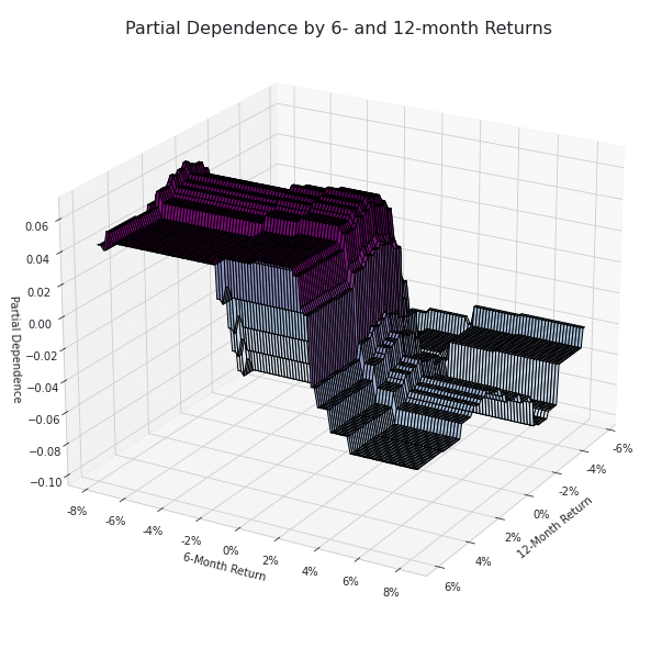
XGBoost
設定
xgb_clf = XGBClassifier(max_depth=3,                  # Maximum tree depth for base learners.
                       learning_rate=0.1,            # Boosting learning rate (xgb's "eta")
                       n_estimators=100,             # Number of boosted trees to fit.
                       silent=True,                  # Whether to print messages while running
                       objective='binary:logistic',  # Task and objective or custom objective function
                       booster='gbtree',             # Select booster: gbtree, gblinear or dart
#                         tree_method='gpu_hist',
                       n_jobs=-1,                    # Number of parallel threads
                       gamma=0,                      # Min loss reduction for further splits
                       min_child_weight=1,           # Min sum of sample weight(hessian) needed
                       max_delta_step=0,             # Max delta step for each tree's weight estimation
                       subsample=1,                  # Subsample ratio of training samples
                       colsample_bytree=1,           # Subsample ratio of cols for each tree
                       colsample_bylevel=1,          # Subsample ratio of cols for each split
                       reg_alpha=0,                  # L1 regularization term on weights
                       reg_lambda=1,                 # L2 regularization term on weights
                       scale_pos_weight=1,           # Balancing class weights
                       base_score=0.5,               # Initial prediction score; global bias
                       random_state=42)              # random seed
交差検証
algo = 'xgboost'fname = results_path / f'{algo}.joblib'
if not Path(fname).exists():
xgb_cv_result, run_time[algo] = run_cv(xgb_clf)
joblib.dump(xgb_cv_result, fname)
else:
xgb_cv_result = joblib.load(fname)結果のプロット
xbg_result = stack_results(xgb_cv_result)
xbg_result.groupby(['Metric', 'Dataset']).Value.mean().unstack()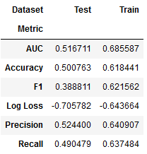
plot_result(xbg_result, model='XG Boost', fname=f'figures/{algo}_cv_result')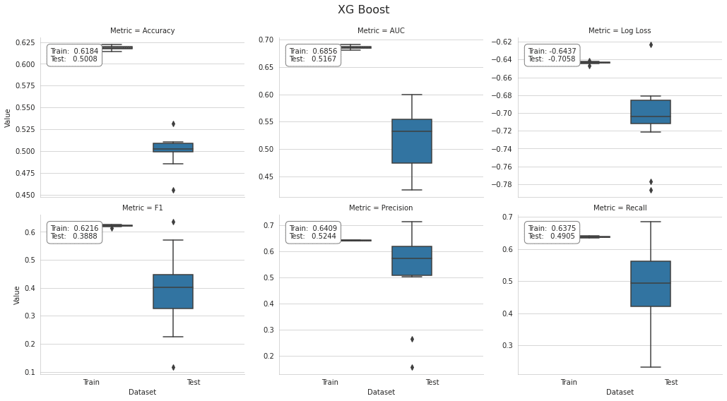
特徴量重要度
xgb_clf.fit(X=X_dummies, y=y)fi = pd.Series(xgb_clf.feature_importances_,
index=X_dummies.columns)fi.nlargest(25).sort_values().plot.barh(figsize=(10, 5),
title='Feature Importance')
sns.despine()
plt.tight_layout();
LightGBM
設定
lgb_clf = LGBMClassifier(boosting_type='gbdt',
#                          device='gpu',
                        objective='binary',          # learning task
                        metric='auc',
                        num_leaves=31,               # Maximum tree leaves for base learners.
                        max_depth=-1,                # Maximum tree depth for base learners, -1 means no limit.
                        learning_rate=0.1,          # Adaptive lr via callback override in .fit() method
                        n_estimators=100,            # Number of boosted trees to fit
                        subsample_for_bin=200000,    # Number of samples for constructing bins.
                        class_weight=None,           # dict, 'balanced' or None
                        min_split_gain=0.0,          # Minimum loss reduction for further split
                        min_child_weight=0.001,      # Minimum sum of instance weight(hessian)
                        min_child_samples=20,        # Minimum number of data need in a child(leaf)
                        subsample=1.0,               # Subsample ratio of training samples
                        subsample_freq=0,            # Frequency of subsampling, <=0: disabled
                        colsample_bytree=1.0,        # Subsampling ratio of features
                        reg_alpha=0.0,               # L1 regularization term on weights
                        reg_lambda=0.0,              # L2 regularization term on weights
                        random_state=42,             # Random number seed; default: C++ seed
                        n_jobs=-1,                   # Number of parallel threads.
                        silent=False,
                        importance_type='gain',      # default: 'split' or 'gain'
                       )
交差検証
カテゴリカル特徴量を用いる
algo = 'lgb_factors'fname = results_path / f'{algo}.joblib'
if not Path(fname).exists():
lgb_factor_cv_result, run_time[algo] = run_cv(lgb_clf, X=X_factors, fit_params={'categorical_feature': cat_cols})
joblib.dump(lgb_factor_cv_result, fname)
else:
lgb_factor_cv_result = joblib.load(fname)プロットの結果
lgb_factor_result = stack_results(lgb_factor_cv_result)
lgb_factor_result.groupby(['Metric', 'Dataset']).Value.mean().unstack()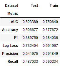
plot_result(lgb_factor_result, model='Light GBM | Factors', fname=f'figures/{algo}_cv_result')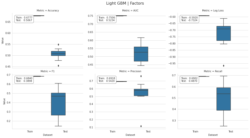
ダミー変数を用いる
algo = 'lgb_dummies'fname = results_path / f'{algo}.joblib'
if not Path(fname).exists():
lgb_dummy_cv_result, run_time[algo] = run_cv(lgb_clf)
joblib.dump(lgb_dummy_cv_result, fname)
else:
lgb_dummy_cv_result = joblib.load(fname)lgb_dummy_result = stack_results(lgb_dummy_cv_result)
lgb_dummy_result.groupby(['Metric', 'Dataset']).Value.mean().unstack()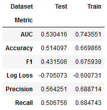
plot_result(lgb_dummy_result, model='Light GBM | Factors', fname=f'figures/{algo}_cv_result')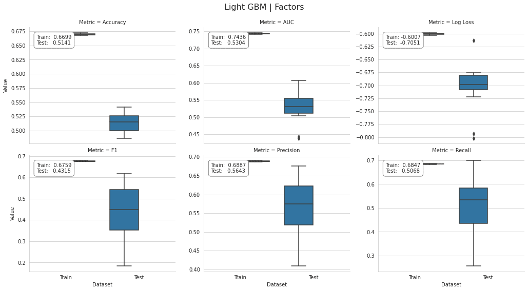
CatBoostClassifier
詳しくはこちら
設定
cat_clf = CatBoostClassifier()交差検証
s = pd.Series(X_factors.columns.tolist())
cat_cols_idx = s[s.isin(cat_cols)].index.tolist()
algo = 'catboost'fname = results_path / f'{algo}.joblib'
if not Path(fname).exists():
cat_cv_result, run_time[algo] = run_cv(cat_clf,
X=X_factors,
fit_params={
'cat_features': cat_cols_idx},
n_jobs=1)
joblib.dump(cat_cv_result, fname)
else:
cat_cv_result = joblib.load(fname)結果のプロット
cat_result = stack_results(cat_cv_result)
cat_result.groupby(['Metric', 'Dataset']).Value.mean().unstack()
plot_result(cat_result, model='CatBoost', fname=f'figures/{algo}_cv_result')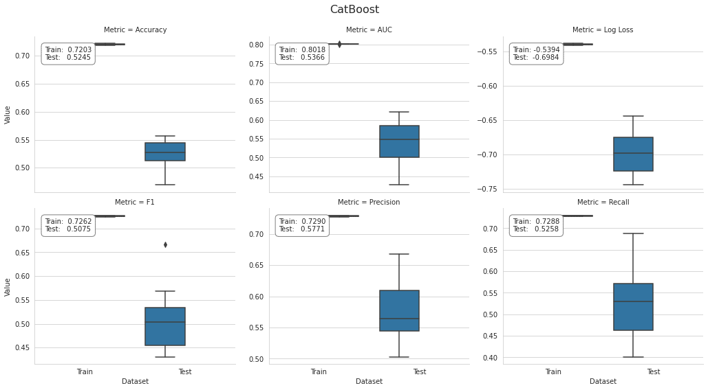
GPU
dockerの環境にGPU入れていなかったので、私はここをスキップしました。
設定
cat_clf_gpu = CatBoostClassifier(task_type='GPU')交差検証
s = pd.Series(X_factors.columns.tolist())
cat_cols_idx = s[s.isin(cat_cols)].index.tolist()
algo = 'catboost_gpu'fname = results_path / f'{algo}.joblib'
if not Path(fname).exists():
cat_gpu_cv_result, run_time[algo] = run_cv(cat_clf_gpu,
X=X_factors,
fit_params={
'cat_features': cat_cols_idx},
n_jobs=1)
joblib.dump(cat_gpu_cv_result, fname)
else:
cat_gpu_cv_result = joblib.load(fname)結果のプロット
cat_gpu_result = stack_results(cat_gpu_cv_result)
cat_gpu_result.groupby(['Metric', 'Dataset']).Value.mean().unstack()
plot_result(cat_gpu_result, model='CatBoost', fname=f'figures/{algo}_cv_result')結果の比較
results = {'Baseline': dummy_result,
          'Random Forest': rf_result,
          'AdaBoost': ada_result,
          'Gradient Booster': gb_result,
          'XGBoost': xbg_result,
          'LightGBM Dummies': lgb_dummy_result,
          'LightGBM Factors': lgb_factor_result,
          'CatBoost': cat_result}
df = pd.DataFrame()
for model, result in results.items():
   df = pd.concat([df, result.groupby(['Metric', 'Dataset']
                                      ).Value.mean().unstack()['Test'].to_frame(model)], axis=1)

df.T.sort_values('AUC', ascending=False)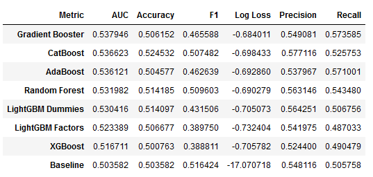
algo_dict = dict(zip(['dummy_clf', 'random_forest', 'adaboost', 'sklearn_gbm',
                     'xgboost', 'lgb_factors', 'lgb_dummies', 'catboost'],
                    ['Baseline', 'Random Forest', 'AdaBoost', 'Gradient Booster',
                     'XGBoost', 'LightGBM Dummies', 'LightGBM Factors', 'CatBoost']))
r = pd.Series(run_time).to_frame('t')
r.index = r.index.to_series().map(algo_dict)
r.to_csv(results_path / 'runtime.csv')auc = pd.concat([v.loc[(v.Dataset=='Test') & (v.Metric=='AUC'), 'Value'].to_frame('AUC').assign(Model=k)
for k, v in results.items()])
auc = auc[auc.Model != 'Baseline']fig, axes = plt.subplots(figsize=(15, 5), ncols=2)
idx = df.T.drop('Baseline')['AUC'].sort_values(ascending=False).index
sns.barplot(x='Model', y='AUC',
data=auc,
order=idx, ax=axes[0])
axes[0].set_xticklabels([c.replace(' ', '\n') for c in idx])
axes[0].set_ylim(.49, .58)
axes[0].set_title('Predictive Accuracy')
(r.sort_values('t')).plot.barh(title='Runtime', ax=axes[1], logx=True, legend=False)
axes[1].set_xlabel('Seconds (log scale)')
sns.despine()
fig.tight_layout();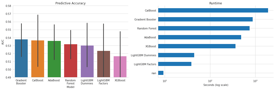
この記事が気に入ったらサポートをしてみませんか?