オープンデータセットとVGGを使って、釣れたアジ、タイ、スズキを認識させる。

2021年5月7日 18:59

ダウンロード

はじめに

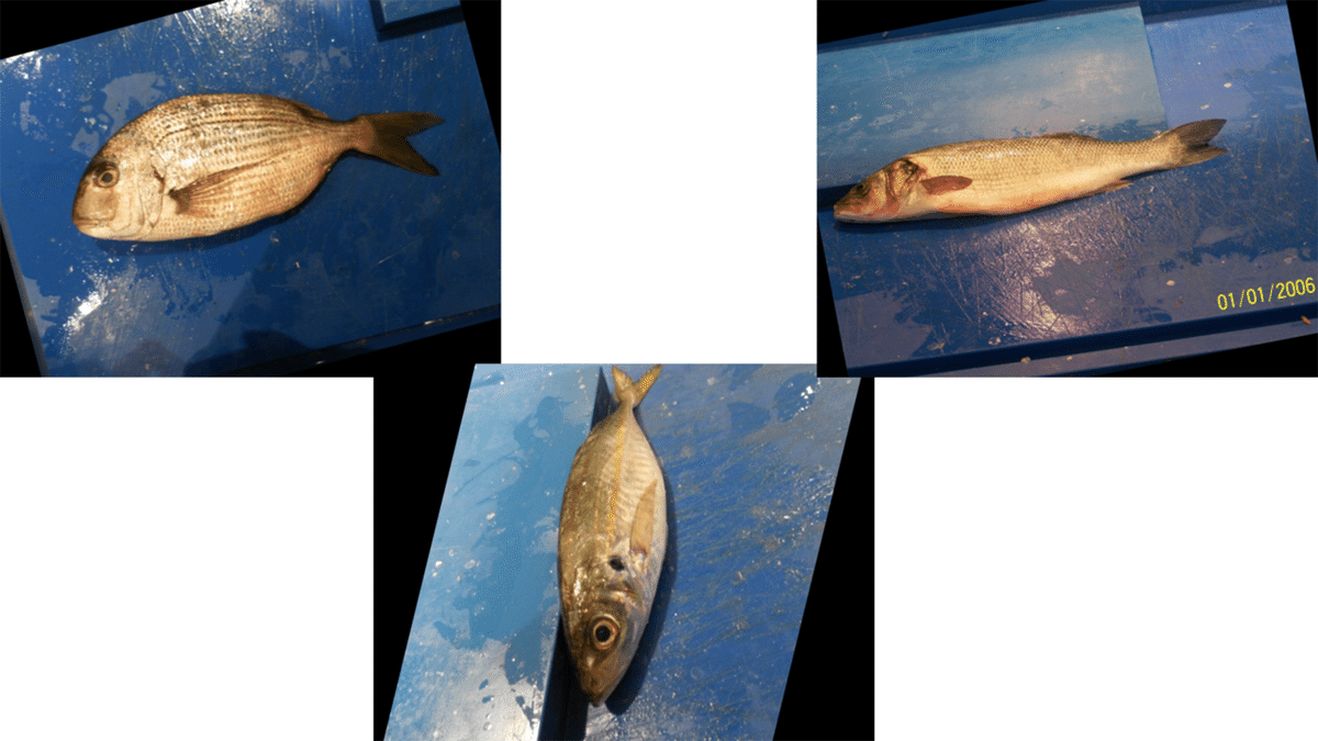
みなさん、釣りに行って、釣れた魚がわからないと思ったことはありませんか。私はよく釣りに行くのですが、そのようなことがたまに起きます。そこで自ら魚を認識できるAIを作成したいと思い、この記事では、アジ、タイ、スズキの３種類の魚を選ばせるAIを作成しました。

オープンデータセットを使用した経緯
当初は、自分で魚のデータを集めようと試みたのですが、釣った状態の魚のデータが思いのほかなく、集めても100枚くらいになってしまったため、各種1000枚あるオープンデータセットを使って魚の画像を集めました。

kaggle - A Large Scale Fish Dataset

- 実装概要
- AIの作成
　　- オープンデータセットの写真を学習/検証データにする
　　- モデルを構築/学習する
　　　　①まずやってみる
　　　　②画像のサイズを変更してみる
　　　　③特徴に注目してshapen変更する
- おわりに

実装概要

Kaggleのオープンデータセット"A Large Scale Fish Dataset"
VGG16を使って転移学習をし、釣れたアジ、タイ、スズキの３種類を認識させます。

AIの作成

オープンデータセットの写真を学習/検証データにする
"A Large Scale Fish Dataset"は海外のものであり、日本では釣れないであろう魚のデータもあったので、今回は日本で釣れる「アジ」「タイ」「スズキ」の３種類だけを抽出しました。
データは1000枚ずつあり、130x130のサイズに変更し、以下のコードでラベリングを実施し、学習、検証データを用意します。
最後に、データ数が3000枚と多いため、毎回処理をしなくてよくするために、pickleを用いてデータセットをdataset.pklというファイルに保存します。

import os, glob
import random, math
import numpy as np
import cv2
import matplotlib.pyplot as plt
import pickle
from keras.applications.vgg16 import VGG16
from keras.optimizers import Adam
from keras.layers import Activation, Dense, Dropout, Flatten, Input
from keras.utils import np_utils
from PIL import Image
from tensorflow.keras.utils import to_categorical
from tensorflow.keras.models import Model, Sequential
from tensorflow.keras import optimizers
from sklearn.model_selection import KFold
from tensorflow.keras.callbacks import EarlyStopping

np.random.seed(0)

# 画像が保存されているルートディレクトリのパス
path_HourseMackerel = os.listdir('パス')
path_RedSeaBream = os.listdir('パス')
path_SeaBass = os.listdir('パス')

# 種類別の魚の画像リスト
img_HourseMackerel = []
img_RedSeaBream = []
img_SeaBass = []

# 画像サイズの横と縦
width = 130
height = 130

# 画像のサイズを変更して各リストに収納
for i in range(len(path_HourseMackerel)):
   img = cv2.imread('パス' + path_HourseMackerel[i])
   img = cv2.resize(img, (width, height))
   img_HourseMackerel.append(img)

for i in range(len(path_RedSeaBream)):
   img = cv2.imread('パス' + path_RedSeaBream[i])
   img = cv2.resize(img, (width, height))
   img_RedSeaBream.append(img)

for i in range(len(path_SeaBass)):
   img = cv2.imread('パス' + path_SeaBass[i])
   img = cv2.resize(img, (width, height))
   img_SeaBass.append(img)

X = np.array(img_HourseMackerel + img_RedSeaBream + img_SeaBass)
y =  np.array([0]*len(img_HourseMackerel) + [1]*len(img_RedSeaBream) + [2]*len(img_SeaBass))

# データセットの保存
with open("datasetの保存先パス/dataset.pkl", "wb") as f:
 pickle.dump((X, y), f)

モデルを構築する/学習する
はじめに、上で保存したdataset.pklからデータセットを読み込みます。
モデルはVGG16を使って、転移学習を行い、モデルを構築します。

# データセットのload
with open("datasetの保存先パス/dataset.pkl", "rb") as f:
 X, y = pickle.load(f)

# VGG16のload
input_tensor = Input(shape=(height, width, 3))
vgg16 = VGG16(include_top=False, weights='imagenet', input_tensor=input_tensor)

# モデルの構築
top_model = Sequential()
top_model.add(Flatten(input_shape=vgg16.output_shape[1:]))
top_model.add(Dense(256, activation='relu'))
top_model.add(Dropout(rate=0.5))
top_model.add(Dense(3, activation='softmax'))

続いて、交差検証（クロスバリデーション）を行います。今回行う、K-分割交差検証は、データをK個に分割してそのうち1つをテストデータに残りのK-1個を学習データとして正解率の評価します。
空のリストである、model_list, loss_list, acc_listを作成し、ここに交差検証の結果を入れ、結果の平均を出力します。最後に、一番良いスコアのモデルmodel.h5として保存します。

# KFoldの定義
kf = KFold(n_splits=3, shuffle=True, random_state=0)

model_list = []
loss_list = []
acc_list = []

# KFoldの実行
for train_index, valid_index in kf.split(X):
   # データの分割
   X_train = X[train_index]
   y_train = y[train_index]
   X_test = X[valid_index]
   y_test = y[valid_index]
   y_train = to_categorical(y_train)
   y_test = to_categorical(y_test)
   
   # モデルの連結
   model = Model(inputs=vgg16.input, outputs=top_model(vgg16.output))
   
   # vgg16の重みの固定
   for layer in model.layers[:19]:
       layer.trainable = False
   
   # 多クラス分類を指定
   model.compile(loss='categorical_crossentropy',
                 optimizer=optimizers.SGD(lr=1e-4, momentum=0.9),
                 metrics=['accuracy'])

   # 学習過程の取得
   callbacks = [EarlyStopping(monitor="val_loss", patience=20)]
   history = model.fit(X_train, y_train, batch_size=100, epochs=100, validation_data=(X_test, y_test), callbacks=callbacks)
   
   # 学習のスコア
   scores = model.evaluate(X_test, y_test, verbose=1)
   model_list.append(model)
   loss_list.append(scores[0])
   acc_list.append(scores[1])

# クロスバリデーションの平均スコアの出力
print('KFold loss mean:', np.mean(loss_list))
print('KFold acc mean:', np.mean(acc_list))

#best_modelの保存
best_score_index = np.argmax(np.array(acc_list))
model_list[best_score_index].save("modelの保存先パス/model.h5")

# 出力結果

Epoch 1/100
21/21 [==============================] - 15s 274ms/step - loss: 12.1657 - accuracy: 0.5927 - val_loss: 0.1465 - val_accuracy: 0.9801
Epoch 2/100
21/21 [==============================] - 4s 190ms/step - loss: 0.6321 - accuracy: 0.9480 - val_loss: 0.0358 - val_accuracy: 0.9930
Epoch 3/100
21/21 [==============================] - 4s 191ms/step - loss: 0.2046 - accuracy: 0.9738 - val_loss: 0.0162 - val_accuracy: 0.9960
Epoch 4/100
21/21 [==============================] - 4s 192ms/step - loss: 0.1170 - accuracy: 0.9831 - val_loss: 0.0176 - val_accuracy: 0.9960
Epoch 5/100
21/21 [==============================] - 4s 191ms/step - loss: 0.0576 - accuracy: 0.9843 - val_loss: 0.0097 - val_accuracy: 0.9960
Epoch 6/100
21/21 [==============================] - 4s 192ms/step - loss: 0.0524 - accuracy: 0.9897 - val_loss: 0.0203 - val_accuracy: 0.9970
Epoch 7/100
21/21 [==============================] - 4s 193ms/step - loss: 0.1353 - accuracy: 0.9814 - val_loss: 0.0212 - val_accuracy: 0.9960
Epoch 8/100
21/21 [==============================] - 4s 194ms/step - loss: 0.1004 - accuracy: 0.9873 - val_loss: 0.0106 - val_accuracy: 0.9980
Epoch 9/100
21/21 [==============================] - 4s 194ms/step - loss: 0.0487 - accuracy: 0.9900 - val_loss: 0.0133 - val_accuracy: 0.9980
Epoch 10/100
21/21 [==============================] - 4s 196ms/step - loss: 0.0357 - accuracy: 0.9934 - val_loss: 0.0055 - val_accuracy: 0.9980

・
・
・

Epoch 25/100
21/21 [==============================] - 5s 228ms/step - loss: 3.8472e-04 - accuracy: 1.0000 - val_loss: 1.1302e-08 - val_accuracy: 1.0000
Epoch 26/100
21/21 [==============================] - 5s 227ms/step - loss: 0.0054 - accuracy: 0.9982 - val_loss: 1.5347e-08 - val_accuracy: 1.0000
Epoch 27/100
21/21 [==============================] - 5s 227ms/step - loss: 7.2735e-04 - accuracy: 1.0000 - val_loss: 1.8678e-08 - val_accuracy: 1.0000
Epoch 28/100
21/21 [==============================] - 5s 228ms/step - loss: 0.0019 - accuracy: 0.9980 - val_loss: 2.2842e-08 - val_accuracy: 1.0000
Epoch 29/100
21/21 [==============================] - 5s 228ms/step - loss: 4.8258e-04 - accuracy: 0.9999 - val_loss: 2.4984e-08 - val_accuracy: 1.0000
Epoch 30/100
21/21 [==============================] - 5s 227ms/step - loss: 0.0014 - accuracy: 0.9989 - val_loss: 3.4382e-08 - val_accuracy: 1.0000
Epoch 31/100
21/21 [==============================] - 5s 227ms/step - loss: 0.0020 - accuracy: 0.9985 - val_loss: 2.8910e-08 - val_accuracy: 1.0000
32/32 [==============================] - 2s 47ms/step - loss: 2.8910e-08 - accuracy: 1.0000
KFold loss mean: 0.0006215953202371635
KFold acc mean: 0.9996676643689474

交差検証の結果、loss平均が0.0006, accuracy平均が0.9996となりました。

①まずやってみる

先ほど保存したmodel.h5を読み込みます。
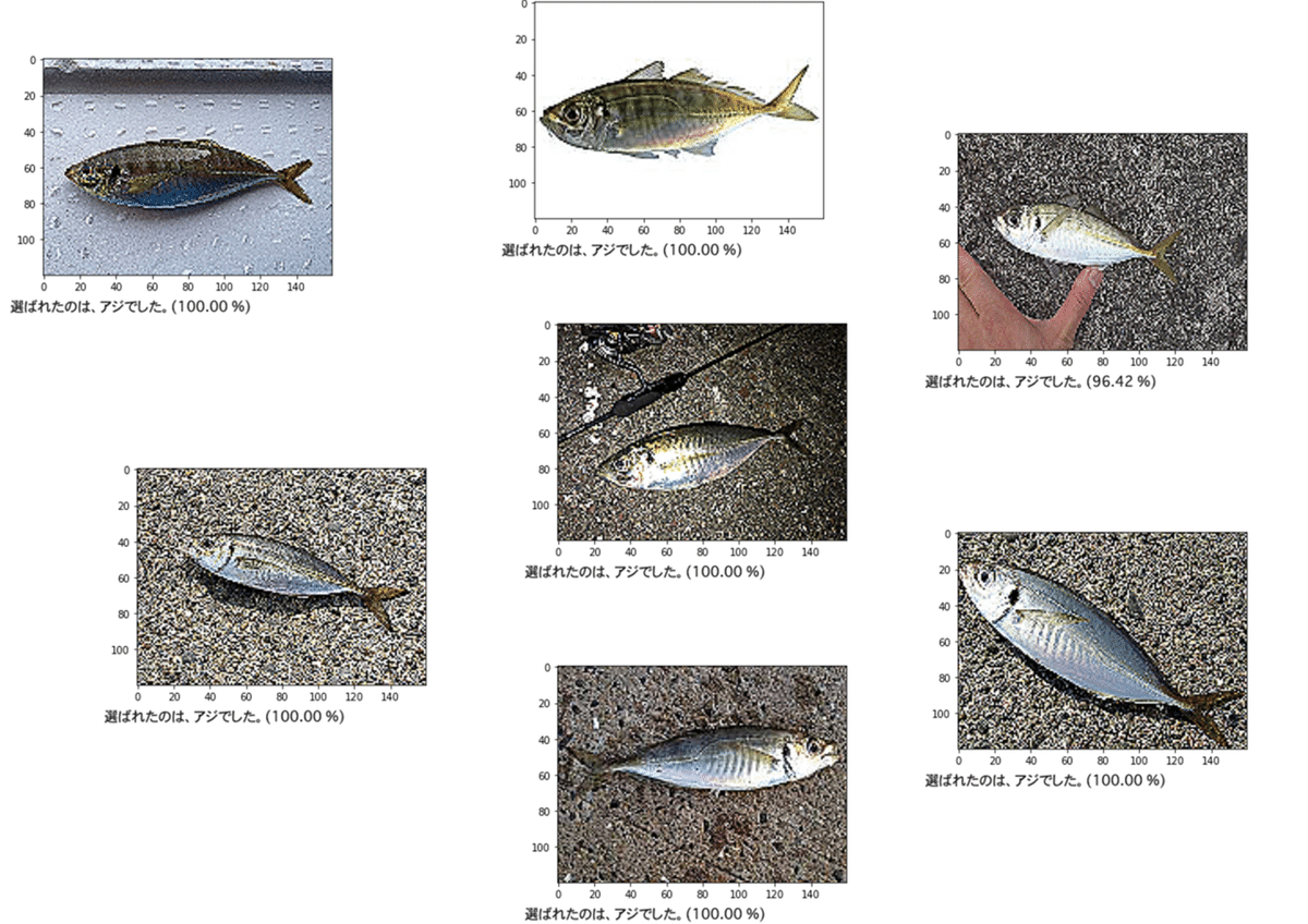
今回評価用写真として、釣ってすぐのような魚の写真をそれぞれ35枚用意しました。（数に意味はありません）
そして、閾値として0.7を指定してあります。これは、どの魚とも断定できなく、70％以上でその魚として認識できなかった時に、「わからなかった」という結果を出力するためのものです。
つまり、70％以上その魚と判定された場合のときだけアジ、タイ、スズキとしての結果が出力されます。
そして、最後にどの魚として判定されたかの確率を出力しています。

from keras.preprocessing import image
from keras.models import load_model

# モデルのload
model = load_model("modelの保存先パス/model.h5")

# 評価用の写真のパス
path_aji = os.listdir('評価用の写真のパス')
path_tai = os.listdir('評価用の写真のパス')
path_suzuki = os.listdir('評価用の写真のパス')

# 画像サイズ
width = 130
height = 130

# 評価精度の計算用
aji_count = 0
tai_count = 0
suzuki_count = 0
other_count = 0

# 閾値
threshold = 0.7

# 魚の分類
comments = ["選ばれたのは、アジでした。", "選ばれたのは、タイでした。", "選ばれたのは、スズキでした。"]

# 評価用の釣り場で撮ったような写真をそれぞれ35枚
for i in range(35):
   #画像を読み込む
   img_path = '評価用の写真のパス'
   img = cv2.imread(img_path + path_aji[i])
   b,g,r = cv2.split(img)
   img = cv2.merge([r,g,b])
   img = cv2.resize(img, (width, height))
   
   # 読み込んだ画像を出力
   plt.imshow(img)
   plt.show()
   
   # 予測
   x = image.img_to_array(img)
   x = np.expand_dims(x, axis=0)
   results = model.predict(x)[0, :]
   
   # 予測結果によって処理を分ける
   if results.max() < threshold:
       print("私にはその魚は、わかりませんでした。"
           + "(アジ: {:.2f} %, ".format(results[0]*100)
           + "タイ: {:.2f} %, ".format(results[1]*100)
           + "スズキ: {:.2f} %)".format(results[2]*100))
       other_count+=1
   else:
       answer_index = np.argmax(results)
       print(comments[answer_index] + "({:.2f} %)".format(results[answer_index]*100))
       if answer_index == 0:
         aji_count+=1
       elif answer_index == 1:
         tai_count+=1
       elif answer_index == 2:
         suzuki_count+=1

# 選ばれた確率
print("(aji: {:.2f} %, ".format(aji_count/35*100)
   +"tai: {:.2f} %, ".format(tai_count/35*100)
   +"suzuki: {:.2f} %, ".format(suzuki_count/35*100)
   +"other: {:.2f} %)".format(other_count/35*100))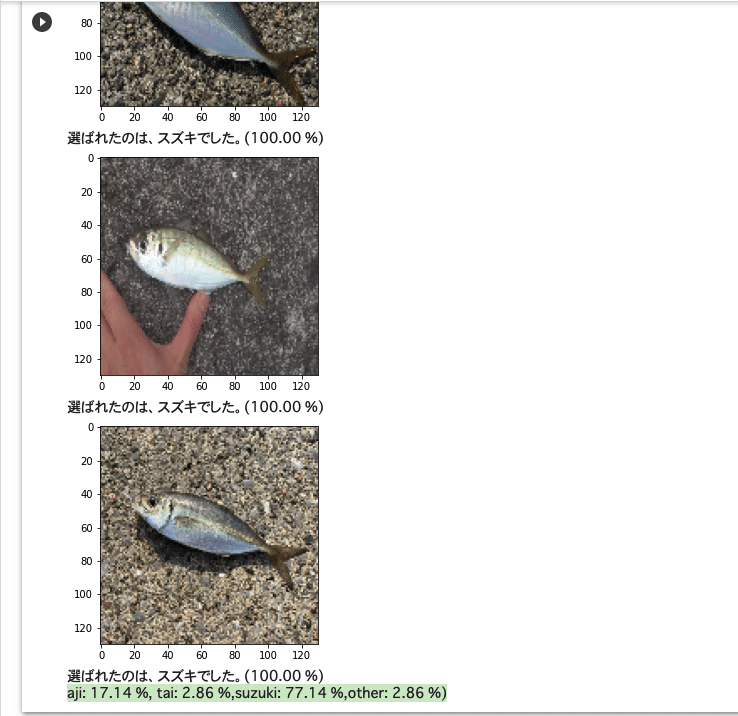

スクリーンショット 2021-05-07 午後6.04.09

実行してみた結果、
アジ - (aji: 17.14 %, tai: 2.86 %, suzuki: 77.14 %,other: 2.86 %)
タイ - (aji: 5.71 %, tai: 68.57 %, suzuki: 22.86 %, other: 2.86 %)
スズキ - (aji: 2.86 %, tai: 0.00 %, suzuki: 97.14 %, other: 0.00 %)
という精度になりました。スズキの精度はかなり良いのですが、アジの精度がかなり悪く、画像を見ると人間から見てもアジの形が太って見えたりしていたので、サイズを変更したら精度が上がるのではないかと考えました。

②画像のサイズを変更してみる
画像サイズを(130,130)から長方形の(160,120)変更しもう一度モデルを構築しました。この画像はmodel2.pklに保存します。

# 画像が保存されているルートディレクトリのパス
path_HourseMackerel = os.listdir('パス')
path_RedSeaBream = os.listdir('パス')
path_SeaBass = os.listdir('パス')

# 種類別の魚の画像リスト
img_HourseMackerel = []
img_RedSeaBream = []
img_SeaBass = []

# 画像サイズの横と縦
width = 160
height = 120

# 画像のサイズを変更して各リストに収納
for i in range(len(path_HourseMackerel)):
   img = cv2.imread('パス' + path_HourseMackerel[i])
   img = cv2.resize(img, (width, height))
   img_HourseMackerel.append(img)

for i in range(len(path_RedSeaBream)):
   img = cv2.imread('パス' + path_RedSeaBream[i])
   img = cv2.resize(img, (width, height))
   img_RedSeaBream.append(img)

for i in range(len(path_SeaBass)):
   img = cv2.imread('パス' + path_SeaBass[i])
   img = cv2.resize(img, (width, height))
   img_SeaBass.append(img)

X = np.array(img_HourseMackerel + img_RedSeaBream + img_SeaBass)
y =  np.array([0]*len(img_HourseMackerel) + [1]*len(img_RedSeaBream) + [2]*len(img_SeaBass))

# データセット2の保存
with open("datasetの保存先パス/dataset２.pkl", "wb") as f:
 pickle.dump((X, y), f)

# データセット2のload
with open("datasetの保存先パス/dataset2.pkl", "rb") as f:
 X, y = pickle.load(f)

前と同様、モデルを構築し、交差検証を行います。
そして今回はmodel2.h5にベストなモデルを保存します。

#best_modelの保存
best_score_index = np.argmax(np.array(acc_list))
model_list[best_score_index].save("modelの保存先パス/model2.h5")

from keras.preprocessing import image
from keras.models import load_model
# モデルのload
model = load_model("modelの保存先パス/model2.h5")

# 評価用の写真のパス
path_aji = os.listdir('評価用の写真のパス')
path_tai = os.listdir('評価用の写真のパス')
path_suzuki = os.listdir('評価用の写真のパス')

# 画像サイズ
width = 160
height = 120

# 評価精度の計算用
aji_count = 0
tai_count = 0
suzuki_count = 0
other_count = 0

# 閾値
threshold = 0.7

# 魚の分類
comments = ["選ばれたのは、アジでした。", "選ばれたのは、タイでした。", "選ばれたのは、スズキでした。"]

# 評価用の釣り場で撮ったような写真をそれぞれ35枚
for i in range(35):
 #画像を読み込む
   img_path = '評価用の写真のパス'
   img = cv2.imread(img_path + path_aji[i])
   b,g,r = cv2.split(img)
   img = cv2.merge([r,g,b])
   img = cv2.resize(img, (width, height))
   # 読み込んだ画像を出力
   plt.imshow(img)
   plt.show()
   # 予測
   x = image.img_to_array(img)
   x = np.expand_dims(x, axis=0)
   results = model.predict(x)[0, :]
   
 
   # 予測結果によって処理を分ける
   if results.max() < threshold:
       print("私にはその魚は、わかりませんでした。"
           + "(アジ: {:.2f} %, ".format(results[0]*100)
           + "タイ: {:.2f} %, ".format(results[1]*100)
           + "スズキ: {:.2f} %)".format(results[2]*100))
       other_count+=1
   else:
       answer_index = np.argmax(results)
       print(comments[answer_index] + "({:.2f} %)".format(results[answer_index]*100))
       if answer_index == 0:
         aji_count+=1
       elif answer_index == 1:
         tai_count+=1
       elif answer_index == 2:
         suzuki_count+=1

# 選ばれた確率
print("(aji: {:.2f} %, ".format(aji_count/35*100)
   +"tai: {:.2f} %, ".format(tai_count/35*100)
   +"suzuki: {:.2f} %, ".format(suzuki_count/35*100)
   +"other: {:.2f} %)".format(other_count/35*100))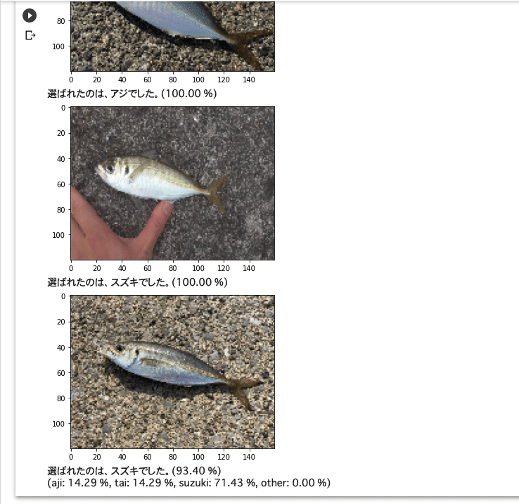

スクリーンショット 2021-05-07 午後6.10.52

実行してみた結果、
アジ - (aji: 14.29 %, tai: 14.29 %, suzuki: 71.43 %, other: 0.00 %)
タイ - (aji: 2.86 %, tai: 77.14 %, suzuki: 20.00 %, other: 0.00 %)
スズキ - (aji: 0.00 %, tai: 0.00 %, suzuki: 100.00 %, other: 0.00 %)

スズキは100％となり、タイの精度も少し上がりました。しかし、アジの精度が下がってしまいました。
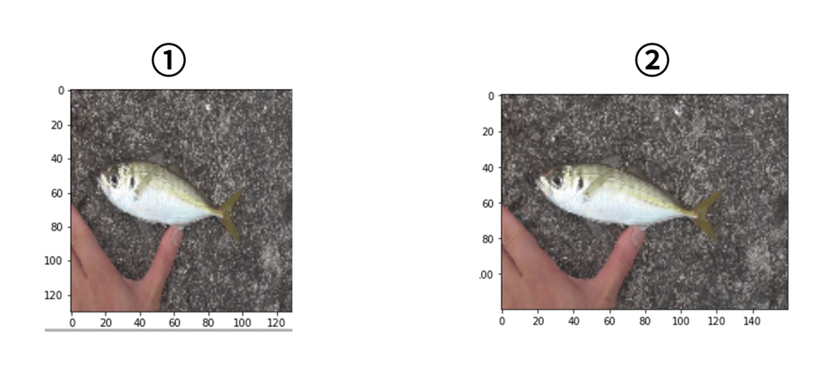
画像サイズを変更したことで、下の画像のように①では太ってみえるのが②では少しスリムになっていることが見てわかると思います。
しかし、アジがほとんどスズキと認識されてしまっているようです。そこで違う方法を考えてみました。

③特徴に注目してshapen（鮮鋭化）する
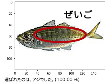
画像サイズを変更してもアジの精度はよくなりませんでした。そこで、アジの特徴の一つであるぜいごを認識しやすくするために、shapen(鮮鋭化)しまし、もう一度モデルを構築しました。
今回は鮮鋭化した画像をdataset3.pklに保存します。

# 画像が保存されているルートディレクトリのパス
path_HourseMackerel = os.listdir('パス')
path_RedSeaBream = os.listdir('パス')
path_SeaBass = os.listdir('パス')

# 種類別の魚の画像リスト
img_HourseMackerel = []
img_RedSeaBream = []
img_SeaBass = []

# 画像サイズの横と縦
width = 160
height = 120

# カーネルの定義
kernel = np.array([[0, -1, 0], [-1, 5, -1], [0, -1, 0]])

# 画像のサイズを変更して各リストに収納
for i in range(len(path_HourseMackerel)):
   img = cv2.imread('パス' + path_HourseMackerel[i])
   img = cv2.resize(img, (width, height))
   
   #sharpen化
   img = cv2.filter2D(img, ddepth=-1, kernel=kernel)
   
   img_HourseMackerel.append(img)

for i in range(len(path_RedSeaBream)):
   img = cv2.imread('パス' + path_RedSeaBream[i])
   img = cv2.resize(img, (width, height))
   
   #sharpen化
   img = cv2.filter2D(img, ddepth=-1, kernel=kernel)
   
   img_RedSeaBream.append(img)

for i in range(len(path_SeaBass)):
   img = cv2.imread('パス' + path_SeaBass[i])
   img = cv2.resize(img, (width, height))
   
   #sharpen化
   img = cv2.filter2D(img, ddepth=-1, kernel=kernel)
   
   img_SeaBass.append(img)

X = np.array(img_HourseMackerel + img_RedSeaBream + img_SeaBass)
y =  np.array([0]*len(img_HourseMackerel) + [1]*len(img_RedSeaBream) + [2]*len(img_SeaBass))

# データセット３の保存
with open("datasetの保存先パス/dataset3.pkl", "wb") as f: pickle.dump((X, y), f)

# データセット3のload
with open("datasetの保存先パス/dataset3.pkl", "rb") as f:
 X, y = pickle.load(f)

#best_modelの保存
best_score_index = np.argmax(np.array(acc_list))
model_list[best_score_index].save("modelの保存先パス/model3.h5")

from keras.preprocessing import image
from keras.models import load_model
# モデルのload
model = load_model("modelの保存先パス/model3.h5")

# 評価用の写真のパス
path_aji = os.listdir('評価用の写真のパス')
path_tai = os.listdir('評価用の写真のパス')
path_suzuki = os.listdir('評価用の写真のパス')

# 画像サイズ
width = 160
height = 120

# 評価精度の計算用
aji_count = 0
tai_count = 0
suzuki_count = 0
other_count = 0

# 閾値
threshold = 0.7

# 魚の分類
comments = ["選ばれたのは、アジでした。", "選ばれたのは、タイでした。", "選ばれたのは、スズキでした。"]

# カーネルの定義
kernel = np.array([[0, -1, 0], [-1, 5, -1], [0, -1, 0]])

# 評価用の釣り場で撮ったような写真をそれぞれ35枚
for i in range(35):
 #画像を読み込む
   img_path = '評価用の写真のパス'
   img = cv2.imread(img_path + path_aji[i])
   b,g,r = cv2.split(img)
   img = cv2.merge([r,g,b])
   img = cv2.resize(img, (width, height))
   
   #sharpen化
   img = cv2.filter2D(img, ddepth=-1, kernel=kernel)
   
   # 読み込んだ画像を出力
   plt.imshow(img)
   plt.show()
   # 予測
   x = image.img_to_array(img)
   x = np.expand_dims(x, axis=0)
   results = model.predict(x)[0, :]
   
 
   # 予測結果によって処理を分ける
   if results.max() < threshold:
       print("私にはその魚は、わかりませんでした。"
           + "(アジ: {:.2f} %, ".format(results[0]*100)
           + "タイ: {:.2f} %, ".format(results[1]*100)
           + "スズキ: {:.2f} %)".format(results[2]*100))
       other_count+=1
   else:
       answer_index = np.argmax(results)
       print(comments[answer_index] + "({:.2f} %)".format(results[answer_index]*100))
       if answer_index == 0:
         aji_count+=1
       elif answer_index == 1:
         tai_count+=1
       elif answer_index == 2:
         suzuki_count+=1

# 選ばれた確率
print("(aji: {:.2f} %, ".format(aji_count/35*100)
   +"tai: {:.2f} %, ".format(tai_count/35*100)
   +"suzuki: {:.2f} %, ".format(suzuki_count/35*100)
   +"other: {:.2f} %)".format(other_count/35*100))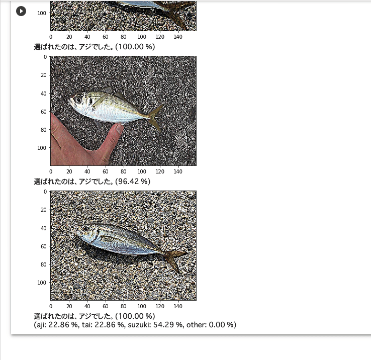

スクリーンショット 2021-05-07 午後6.51.02

実行してみた結果、
アジ - (aji: 22.86 %, tai: 22.86 %, suzuki: 54.29 %, other: 0.00 %)
タイ - (aji: 0.00 %, tai: 85.71 %, suzuki: 14.29 %, other: 0.00 %)
スズキ - (aji: 11.43 %, tai: 17.14 %, suzuki: 71.43 %, other: 0.00 %)

アジの精度は8%ほどあがっていました。実際に画像を見ているとアジと認識されている写真は、ぜいごが尾から中心くらいまでまっすぐ伸びていて、顔に向かって曲線を描いているように見えるものが多い気がしました。

おわりに

オープンデータセットとVGGを使用することによって、私のようなプログラミング初心者でもこのような画像認識をすることができました。
アジの精度はまだまだ低いですが、スズキやタイの精度はそこそこ高いものにすることができました。これからアジの精度を上げるために色々工夫していきたいと思います。

今後もPython, AI, データサイエンスの勉強を続けていき、いつかは業務で使えるようなAIシステムを作りたいと考えています。

※記事にミスや改善点等ございましたら、ご指摘いただけると幸いです。

この記事が気に入ったらサポートをしてみませんか？

オープンデータセットとVGGを使って、釣れたアジ、タイ、スズキを認識させる。

はじめに

目次

実装概要

AIの作成

おわりに