ネットワークのモジュラー中心性を調べてみた。

2023年2月6日 17:10

こんばんは。最近、「Centrality in modular networks」という論文を読んで、その中に、モジュラー中心性を求めるアルゴリズムが記載されていました。そのため、Chat GPTを利用しながら、このアルゴリズムをRのコードに書き直し、トイモデルで実験しました。自分の整理を兼ねて数回に分けてAlgorithm 1: Generic computation of Modular centralityのコードを掲載していこうと思います。

背景

（疫学に興味があるので、感染症に限定した内容になります。）ネットワーク上の影響力あるノード（個人や施設）を特定することで、感染症の広がりを止めることにつながります。これまでに次数中心性、媒介中心性及び固有値に基づく中心性などの指標を用いて、ネットワークに影響を持つ個体を特定する研究がされてきました。しかし、実はネットワークは満遍なく個体が繋がっていることは少なく、１つの大きなネットワークに密に繋がっている領域があります。これをコミュニティと呼ばれることがあります。こうした密な領域と疎な領域がある構造をモジュラー構造とこの論文では呼んでいます。最近の研究では、このモジュラー構造がネットワークの動態に大きく影響することがわかっています。この論文では、ノードが持つ影響について２つに分類しています：所属するコミュニティ内の他のノードに対するローカルな影響と、他のコミュニティ内のノードに対するグローバルな影響。この２つの指標を二次元のベクトルと見做し、モジュラー構造を持つネットワークへの適用について検討したというのがこの論文の前半に当たります。論文の後半ではSIRモデルへの拡張も検証しており、こちらは今回触れません。

準備

パッケージはigraphを使います。

# Load packages
library(igraph)


# set seed number

set.seed(2023)

トイモデルの作成

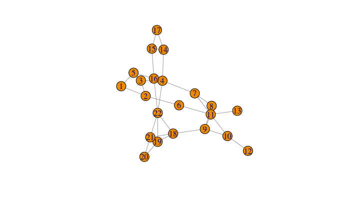
G(V,E)=(22, 34)の無方向性のグラフです。これを以後Gと呼ぶことにします。

# Create a toy graph: g
g<-　graph_from_edgelist(
    matrix(
       c(
         1,2,
         1,5,
         2,3,
         2,6,
         3,4,
         3,5,
         4,5,
         4,7,
         4,14,
         4,16,
         4,22,
         6,11,
         7,8,
         7,11,
         8,9,
         8,11,
         9,10,
         9,11,
         9,18,
         10,11,
         10,12,
         11,13,
         14,15,
         14,17,
         15,16,
         15,17,
         16,22,
         18,19,
         18,21,
         18,22,
         19,20,
         19,22,
         20,21,
         21,22
         ),
       ncol=2,
       byrow = TRUE),
     directed = FALSE)
plot(g)

Gのプロット

ステップ1：中心性指標の選択

ここでは、媒介中心性betweenness centralityを選択しました。

ステップ2：オリジナルのネットワークGからコミュニティ間を結ぶノードを除去及び各コミュニティのローカルな指標（βローカル）を計算

「Infomap」を使って、グラフ「G」からコミュニティを検出し、各コミュニティをサブグラフとして保存します。また、各コミュニティの媒介中心性と次数を計算し、各サブグラフのノードの変数に格納します。

# Calculate communities in the graph
communities <- cluster_infomap(g)

# Add community information to the original graph
V(g)$community <-communities$membership

# Create a list to store subgraphs for each community
l.subgraphs <- list()

# Loop through each community
for (i in unique(communities$membership)) {
  
# Extract the nodes in the current community
  community_nodes <- which(communities$membership == i)
  
# Create a subgraph for the current community
  l.subgraphs[[i]] <- induced_subgraph(g, community_nodes)
  
# Calculate the betweenness centrality for the subgraph
  betweenness_centrality <- betweenness(l.subgraphs[[i]])
  degree_num<- degree(l.subgraphs[[i]])
  
# Add the betweenness centrality as a new vertex attribute to the subgraph
  V(l.subgraphs[[i]])$l.betweenness_centrality <- betweenness_centrality
  
# This code is for the calculation of inter community links in the later step
  V(l.subgraphs[[i]])$l.degree <- degree_num 
}

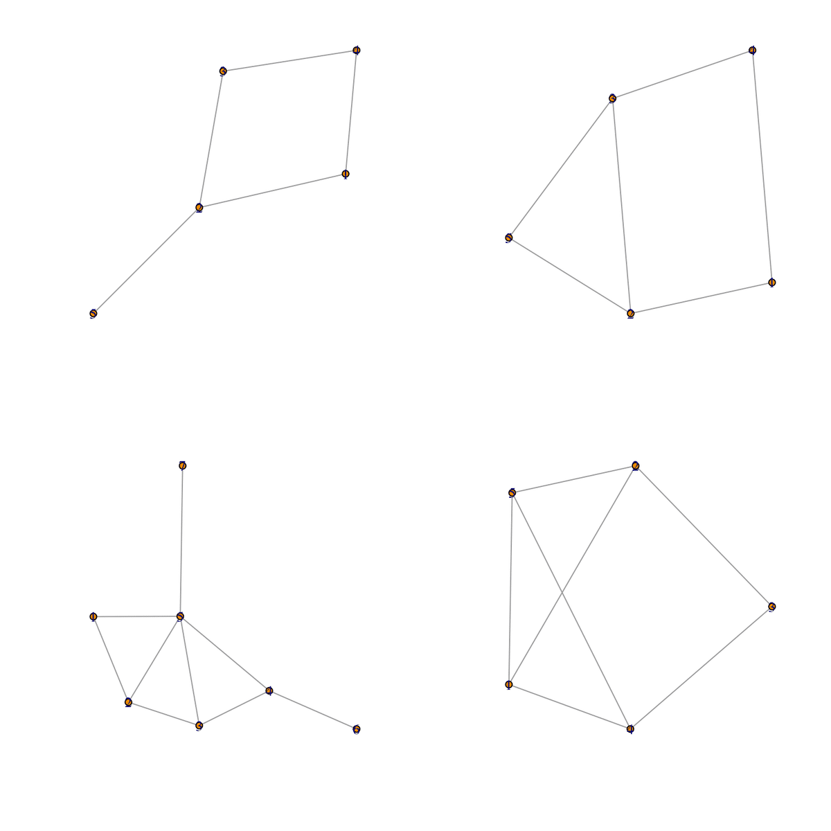
各コミュニティのプロット

４つのコミュニティに分割されました。

ステップ３：各コミュニティのローカルな指標（βローカル）をオリジナルのグラフGに格納する。

ここはChat GPTに手伝って貰いました。とはいえかなり手を加えています。

# Initialize a vector to store the degree centrality values for the original graph
local_betweenness_centrality_vector <- numeric(vcount(g))
local_degree_vector <- numeric(vcount(g))

# Loop through the subgraphs
for (i in l.subgraphs) {
  # Get the node indices of the current subgraph in the original graph
  node_indices <- which( V(g)$community %in% (V(i)$community))

  # Extract the degree centrality values for each node in the subgraph
  subgraph_betweenness_centrality <- V(i)$l.betweenness_centrality
  subgraph_degree <- V(i)$l.degree
  
  # Assign the degree centrality values to the corresponding nodes in the original graph
  local_betweenness_centrality_vector[node_indices] <- subgraph_betweenness_centrality
  local_degree_vector[node_indices]<-subgraph_degree
}

# Add the degree centrality values to the original graph as a node attribute
V(g)$local_betweenness_centrality <- local_betweenness_centrality_vector
V(g)$local_degree                 <- local_degree_vector

ステップ4：Gからコミュニティ内のエッジを除去し、つながりのあるサブグラフ（Gグローバル）を作成

ここから、論文の着目点であるモジュラー中心性に話が映ります。

# Edges that do not across the communities
intra_community_edges<-E(g)[!igraph::crossing(communities, g)]

# Remove the intra-community edges
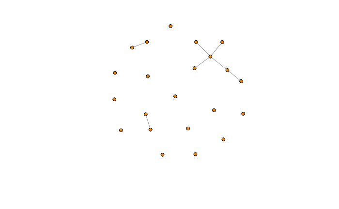
g.sub<- delete_edges(g, intra_community_edges)

Gグローバルのプロット

コミュニテイ間のエッジを取り除いたので、夏の大三角形みたいなグラフになりました。ステップ４で得られたサブグラフを、コミュニティと区別するため、使用したcomponent()に因み、コンポーネントと呼ぶことにします。コンポーネントはグローバル指標の計算に用います。

ステップ6：各コンポーネントのグローバル指標（βグローバル）の計算

# Calculate the connected components of the graph
components <- components(g.sub)

# Add component information to the original graph

V(g)$components <-components$membership

# Create a list to store subgraphs for each connected component
g.subgraphs <- list()

# Loop through each connected component
for (i in 1:max(components$membership)) {
  # Extract the nodes in the current component
  component_nodes <- which(components$membership == i)
  
  # Create a subgraph for the current component
  g.subgraphs[[i]] <- induced_subgraph(g, component_nodes)
  
  # Calculate the betweenness centrality for the subgraph
  betweenness_centrality <- betweenness(g.subgraphs[[i]])
  
  # Add the betweenness centrality as a new vertex attribute to the subgraph
  V(g.subgraphs[[i]])$g.betweenness_centrality <- betweenness_centrality
}

ステップ７：各コンポーネントのβグローバルをオリジナルのグラフGに格納する。

# Initialize a vector to store the degree centrality values for the original graph

global_betweenness_centrality_vector <- numeric(vcount(g))

# Loop through the subgraphs
for (i in g.subgraphs){
  # Get the node indices of the current subgraph in the original graph
  node_indices <- which(V(g)$components %in% (V(i)$components))
 
  # Extract the degree centrality values for each node in the subgraph
  subgraph_betweenness_centrality <- V(i)$g.betweenness_centrality

  # Assign the degree centrality values to the corresponding nodes in the original graph
  global_betweenness_centrality_vector[node_indices] <- subgraph_betweenness_centrality
}

# Add the degree centrality values to the original graph as a node attribute
V(g)$global_betweenness_centrality <- global_betweenness_centrality_vector

これでオリジナルのグラフGにローカル及びグローバル指標を格納することができました。

モジュラー中心性のランキング方法

これまでに求めた２つの指標：ローカル及びグローバルの中心性を用いて、新しい変数を作っていきます。ここで作成した新しい変数を元に他のノードに及ぼす影響を順位付けていきます。論文では４つの変数が提案されています。このページでは３つ紹介します。

Modulus

ローカルとグローバルを２次元のベクトルと見做し、ユークリッド距離に変換する方法のようです。

V(g)$modulus<-sqrt(V(g)$local_betweenness_centrality^2+V(g)$global_betweenness_centrality^2)

アークタンジェント

V(g)$arctan<-atan(V(g)$global_betweenness_centrality/V(g)$local_betweenness_centrality)

タンジェント

V(g)$tan<-tan(V(g)$global_betweenness_centrality/V(g)$local_betweenness_centrality)

残り１つの重み付けモジュラー指標αの説明は次回以降にします。

参考文献

Ghalmane, Z., El Hassouni, M., Cherifi, C. et al. Centrality in modular networks. EPJ Data Sci. 8, 15 (2019). https://doi.org/10.1140/epjds/s13688-019-0195-7

この記事が気に入ったらサポートをしてみませんか？