Python機械学習(GBDT)：XGBoost

記載内容が多くなる＋とりあえず使いたいため作成＝＞追って追記予定

１．概要

　今回はGradient Boosting Decision Tree勾配ブースティング決定木の一つであるXGBoostを紹介します。

Python Package Introduction — xgboost 1.5.1 documentation

XGBoost: A Scalable Tree Boosting System

２．XGBoostについて

２－１．モデルの概要・特徴

　Gradient Boosting Decision Tree（GBDT）は下記手法を組み合わたモデルであり、テーブルデータ表形式に強いため多次元データの回帰・分類分析に向いています。

●勾配降下法(Gradient)
●Boosting(アンサンブル)
●決定木(Decision Tree)

　GBDTの特徴としては下記があります。

★数値の大きさスケーリングはモデルで補正されるため正規化数値の前処理しなくてもよい
●欠損値があってもそのまま処理が可能である。
●分岐の繰り返しで変数間の相互作用を反映：One-hot Encodingだけでなく、Label Encodingでも十分な精度が出る。

　なおGBDTは高精度が期待されるモデルですが高精度を目指すにはデータの特徴量を作ることが重要になります不要な項目を抜いたり、新しく追加したりなど。

２－２．データ構造：DMatrix

追って

２－３．API：Learning API/Scikit-Learn API

 　XGBoostのAPIはLearning APIとScikit Learn APIの2種あります書き方が2通り。基本的には好きな方でよいと思います。

Python API Reference — xgboost 1.5.1 documentation

２－４．設定用パラメータ

　XGBoostをインスタンス化時に使用するパラメータは下記の通りです。

【XGBoostのパラメータ】
●silent：1にすることで学習時に出てくる表示をなくすことができる。
●eval_metric：損失関数（目的関数）の設定
●tree_method(※GPU可)：exact/ gpu exact
●objective{default=reg:squarederror}：学習方法の設定(下記は主要一覧)
　->reg:squarederror: regression with squared loss.
　->reg:squaredlogerror: regression with squared log loss
　->reg:logistic: logistic regression.
　->binary:logistic: 2値の分類のlogistic regression, output probability
　->multi:softmax: set XGBoost to do multiclass classification
●predictor(※GPU可)： cpu_predictor/gpu_predictor

２－５．ハイパーパラメーター

　XGBoostで調整するハイパーパラメータの一部を紹介します。

【XGBoostのハイパーパラメータ】
●booster(ブースター)：gbtree(デフォルト), gbliner, dartの3種から設定
　->gblinearは線形モデル、dartはdropoutを適用します。
●eta(学習率lr){defalut:0.3}：学習時の重みの更新率を調整
　->lrを小さくし決定木の数を増やすと精度向上が見込めるが時間がかかる
●n_estimators：決定技の数
●min_child_weight{defalut:1}：決定木の葉の重みの下限
　->小さいほど過学習寄り（0.1~10.0くらいで調整）
●max_depth{defalut:6}：木構造の深さ
　->深いほど表現力は高いが過学習となる（3~9くらいで調整）
●subsample{defalut:1}：決定木ごとの訓練データからのサンプリング割合
　->ランダム性が入る：過学習時に値を減らしてみる(0.6~0.95)　
●gamma{defalut:0}：決定木の葉ノードを分岐させるために必要なも目的変数の最小値：値が大きくなると分岐しにくくなる
●alpha{defalut:0}：決定木の葉ノードの重みに対するL1正則化の強度
●lambda{defalut:1}：決定木の葉ノードの重みに対するL2正則化の強度

XGBoost公式：XGBoost Parameters、Notes on Parameter Tuning

【XGBoost.cv()メソッドのハイパーパラメータ】
●num_boost_round {defalut:10}：決定木の数（Boostingの反復回数）
　->値を1000のように大きめにしてEarly stoppingと併用すると便利
●early_stopping_rounds{defalut:None}：Early stoppingの監視回数
　->設定するならとりあえず50くらいにしておいて、後で調整

３．Learning API

　追って

４．Scikit-Learn API

　サンプルデータを使用してXGBoostを使用してみます。サンプルデータは下記のとおりです。通常は特徴量エンジニアリングをしますが今回はデータをそのまま使用します。

[In]
import sklearn.datasets as datasets
import pandas as pd
from sklearn.model_selection import train_test_split

cancer = datasets.load_breast_cancer() #分類データ(Classification)

def make_data(data, dftype = True):
    X, y = data.data, data.target
    columns = data.feature_names
    if dftype:
        X = pd.DataFrame(X, columns=columns)
        y = pd.DataFrame(y, columns=['target'])
    return X, y

def split_data(X: pd.DataFrame, y: pd.DataFrame, test_size: float = 0.3, random_state: int = 0):
    X_train, X_test, y_train, y_test = train_test_split(X, y, test_size=test_size, random_state=random_state)
    return X_train, X_test, y_train, y_test


X, y = make_data(cancer)
X_train, X_test, y_train, y_test = split_data(X, y)
print('Cancer data：','X_train.shape', X_train.shape, 'X_test.shape', X_test.shape, 'y_train.shape', y_train.shape, 'y_test.shape', y_test.shape)

[Out]
Cancer data： X_train.shape (398, 30) X_test.shape (171, 30) y_train.shape (398, 1) y_test.shape (171, 1)

４－１．分類分析：XGBClassifier

　分類問題を解く場合Cancerデータは2値分類は下記のとおりです。精度は96%でそれなりに良いです。

[In]
import xgboost as xgb
from sklearn.metrics import confusion_matrix
import seaborn as sns
import matplotlib.pyplot as plt
import japanize_matplotlib


#モデルの作成・学習・評価
model = xgb.XGBClassifier(random_state=0) #XGBoostの分類モデルを作成
model.fit(X_train, y_train) #学習
y_pred = model.predict(X_test) #予測
score = model.score(X_test, y_test) #正解率
print(f'score{score:.2f}')

#混合行列(Confusion Matrix)
matrix = confusion_matrix(y_test, y_pred) 
matrix = pd.DataFrame(matrix, columns=['0:悪性', '1:良性'], index=['0:悪性', '1:良性'])
plt.figure(figsize=(6,6))
sns.heatmap(matrix, annot=True, fmt='d', cmap='Blues', cbar=False)

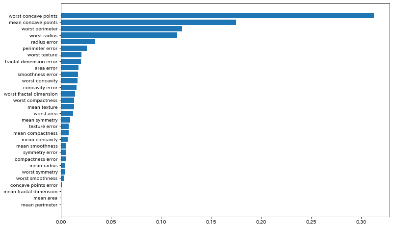
#重要度分析
importance = model.feature_importances_
df_imp = pd.Series(importance, index=X_train.columns).sort_values(ascending=True)
plt.figure(figsize=(12,6))
plt.barh(df_imp.index, df_imp)

[Out]
score0.96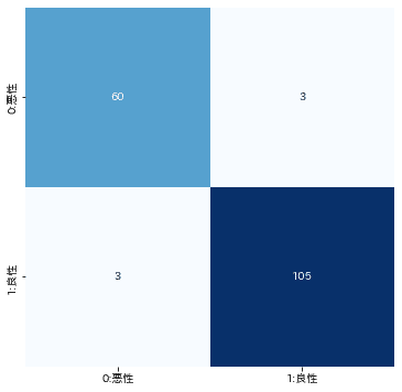

４－２．回帰分析：XGBRegressor

　回帰分析出力値が数値の場合は下記のとおりです。分類問題のScoreは精度(正解数÷データ数)ですが下記の回帰分析ではMSEのため平均二乗誤差参考値です。
　下記より今回は十分な精度が出ていないことが確認されました。(特徴量が不十分かも?)

[In]
from sklearn.metrics import r2_score

diabetes = datasets.load_diabetes() #回帰データ(Regression)
X, y = make_data(diabetes)
X_train, X_test, y_train, y_test = split_data(X, y)
print('Cancer data：','X_train.shape', X_train.shape, 'X_test.shape', X_test.shape, 'y_train.shape', y_train.shape, 'y_test.shape', y_test.shape)

#モデルの作成・学習・評価
model = xgb.XGBRegressor(objective = 'reg:squarederror', random_state=0) #XGBoostの分類モデルを作成
model.fit(X_train, y_train) #学習
y_pred = model.predict(X_test) #予測
score = model.score(X_test, y_test) #正解率
print(f'score(MSE){score:.3f}', f'r2_score{r2_score(y_test, y_pred):.3f}') #SCOREはR2値(決定係数)と同じであることを確認

#予測精度の可視化
plt.figure(figsize=(6,6))
plt.scatter(y_test, y_pred)
plt.plot([0, y_test.max()], [0, y_test.max()], c='k')
plt.xlabel('y_test(正解値)'); plt.ylabel('y_pred(予測値)')
plt.grid()

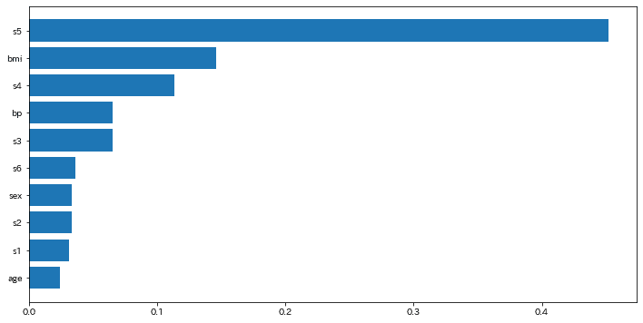
#重要度分析
importance = model.feature_importances_
df_imp = pd.Series(importance, index=X_train.columns).sort_values(ascending=True)
plt.figure(figsize=(12,6))
plt.barh(df_imp.index, df_imp)

[Out]
Cancer data： X_train.shape (309, 10) X_test.shape (133, 10) y_train.shape (309, 1) y_test.shape (133, 1)
score(MSE)0.246 r2_score0.246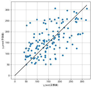

４ー３．ハイパーパラメータの調整：グリッドサーチ

　XGBoostのハイパーパラメータを調整して最適解を探っていきます。

[In1]
from sklearn.model_selection import GridSearchCV

params ={'max_depth':[3,5,7],
            'min_child_weight':[1.0, 2.0, 4.0],
            }

#モデルの作成・学習・評価
model = xgb.XGBRegressor(objective = 'reg:squarederror', tree_method='gpu_hist' , random_state=0) #XGBoostの分類モデルを作成

model_grid = GridSearchCV(model, params, cv=5)

model_grid.fit(X_train,
                y_train,
                early_stopping_rounds=50,
                eval_set=[(X_train, y_train)],
                verbose=0)

[In2]
model_best = model_grid.best_estimator_
y_pred = model_best.predict(X_test) #予測
score = model_best.score(X_test, y_test) #正解率
print(f'score(MSE){score:.2f}')

#予測精度の可視化
plt.figure(figsize=(6,6))
plt.scatter(y_test, y_pred)
plt.plot([0, y_test.max()], [0, y_test.max()], c='k')
plt.xlabel('y_test(正解値)'); plt.ylabel('y_pred(予測値)')
plt.grid()

#重要度分析
importance = model_best.feature_importances_
df_imp = pd.Series(importance, index=X_train.columns).sort_values(ascending=True)
plt.figure(figsize=(12,6))
plt.barh(df_imp.index, df_imp)

[Out]
score(MSE)0.14

　精度が落ちたけどなんでだろう・・・・・(細かい部分は追って確認)

５．精度向上のコツ

５－１．ハイパーパラメータ調整

　XGBoostと同じGBDTモデルであるLightGBMの公式Docs：For Better Accuradyより、ハイパーパラメータ調整のコツは下記の通りです。

1. Use large max_bin (may be slower):大きめのmax_bin使用

2. Use small learning_rate with large num_iterations:小さめの学習率使用

3. Use large num_leaves (may cause over-fitting):大きめのnum_leaves使用

4. Use bigger training data:大量の学習データを使用

   • 1, 3で表現力が向上する反面、過学習の恐れがあるためデータ数が必要

5. Try dart:dartを使用

Parameters Tuning — LightGBM 4.0.0.99 documentation

---

参考資料

●Complete Guide to Parameter Tuning in XGBoost with codes in Python

なぜn_estimatorsやepochsをパラメータサーチしてはいけないのか - 天色グラフィティ

20 Burning XGBoost FAQs Answered to Use the Library Like a Pro

株で儲けたい-最適なハイパーパラメータを見つける | データ駆動はじめ

Distributed XGBoost with Dask — xgboost 1.6.1 documentation

Scale XGBoost — Dask Examples documentation

Python: SHAP (SHapley Additive exPlanations) を LightGBM と使ってみる - CUBE SUGAR CONTAINER

---

あとがき

　XGBoostはDMatrixという型で処理しているが、PandasのDataFrameで直接処理が可能である。ただここら辺のまとまりが十分に理解できていないため、作りながら体裁をまとめていきたいです。

【追加内容】

• 調整できるハイパーパラメータの追加

• CPUとGPUの切り替え

• DMatrixとPandas使用での差異

• 可視化＝＞複数の木構造をまとめて出力（参考用）

　ずっと独学でやって実装した後に下記本を読んだのだけどもっと早く出会えたらよかった。

Kaggleで勝つデータ分析の技術