
第6章 第一節 機械学習ワークフロー

こんにちは、今回は機械学習ワークフローについて解説していきたいと思います。
今回はsklearnを中心に使います。
内容としましては、
1.機械学習の予測の種類(回帰と分類)
2.それぞれ簡単なモデルを利用して、ハイパーパラメーターチューニング
3.予測結果の評価
に分けて説明しております。
k-nearest Neighborsとは
本記事には、住宅価格のデータセットを使用した機械学習ワークフローを示すいくつかの例が含まれています。
回帰と分類の両方の問題に取り組むことができるかなり単純なk近傍法(KNN)アルゴリズムを使用します。
デフォルトのsklearn実装では、(ユークリッド距離に基づいて)k個の最も近いデータポイントを識別して予測を行います。これは、近傍内で最も頻度の高いクラス、または分類または回帰の場合の平均結果をそれぞれ予測します。
インポートと設定
import warnings
warnings.filterwarnings('ignore')
%matplotlib inline
from pathlib import Path
import numpy as np
import pandas as pd
import seaborn as sns
import matplotlib.pyplot as plt
from scipy.stats import spearmanr
from sklearn.neighbors import (KNeighborsClassifier,
KNeighborsRegressor)
from sklearn.model_selection import (cross_val_score,
cross_val_predict,
GridSearchCV)
from sklearn.feature_selection import mutual_info_regression
from sklearn.preprocessing import StandardScaler, scale
from sklearn.pipeline import Pipeline
from sklearn.metrics import make_scorer
from yellowbrick.model_selection import ValidationCurve, LearningCurvesns.set_style('whitegrid')データ取得
Kaggleからのデータになります。
以下の通りAPIを使用してダウンロードすることも可能です。
kaggle datasets download -d harlfoxem/housesalespredictionDATA_PATH = Path('..', 'data')house_sales = pd.read_csv('kc_house_data.csv')
house_sales = house_sales.drop(
['id', 'zipcode', 'lat', 'long', 'date'], axis=1)
house_sales.info()
'''
<class 'pandas.core.frame.DataFrame'>
RangeIndex: 21613 entries, 0 to 21612
Data columns (total 16 columns):
price 21613 non-null float64
bedrooms 21613 non-null int64
bathrooms 21613 non-null float64
sqft_living 21613 non-null int64
sqft_lot 21613 non-null int64
floors 21613 non-null float64
waterfront 21613 non-null int64
view 21613 non-null int64
condition 21613 non-null int64
grade 21613 non-null int64
sqft_above 21613 non-null int64
sqft_basement 21613 non-null int64
yr_built 21613 non-null int64
yr_renovated 21613 non-null int64
sqft_living15 21613 non-null int64
sqft_lot15 21613 non-null int64
dtypes: float64(3), int64(13)
memory usage: 2.6 MB
'''特徴量を選択&変換
まずは、住宅価格の分布について見ていきましょう。
sns.distplot(house_sales.price)
sns.despine()
plt.tight_layout();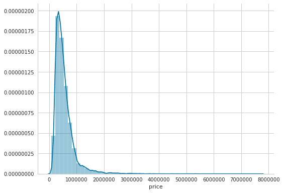
おやおや、見たことあるような分布ですね。対数正規分布に近い形をしております。スキューを直すために、対数変換します。
X_all = house_sales.drop('price', axis=1)
y = np.log(house_sales.price)
相互情報回帰
翻訳の方法が分からなかったですが、こちらsklearnを参考にします。
2つの確率変数間の相互情報(MI)は、変数間の依存関係を測定する非負の値です。 「MIが0になること」と「2つの確率変数が独立であること」は同値であり、高いMIの値は高い依存性を示します。
まずは素直にsklearnを用いて、相互情報回帰をフィッティングしましょう。
mi_reg = pd.Series(mutual_info_regression(X_all, y),
                  index=X_all.columns).sort_values(ascending=False)
mi_reg
'''
sqft_living      0.348555
grade            0.343704
sqft_living15    0.272196
sqft_above       0.259758
bathrooms        0.209994
sqft_lot15       0.085906
bedrooms         0.080822
yr_built         0.074505
floors           0.073565
sqft_basement    0.065731
sqft_lot         0.062601
view             0.054386
waterfront       0.015364
condition        0.011963
yr_renovated     0.009406
dtype: float64
'''
上位10個の特徴量について見ていきます。
X = X_all.loc[:, mi_reg.iloc[:10].index]g = sns.pairplot(X.assign(price=y), y_vars=['price'], x_vars=X.columns)
sns.despine();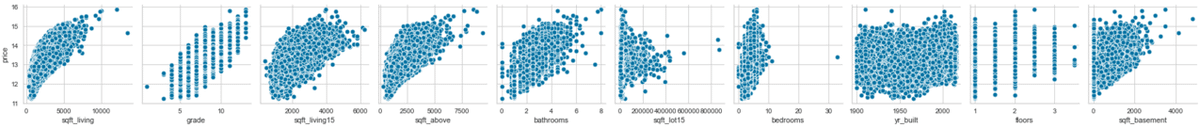
相関関係を見る
correl = (X
         .apply(lambda x: spearmanr(x, y))
         .apply(pd.Series, index=['r', 'pval']))

correl.r.sort_values().plot.barh();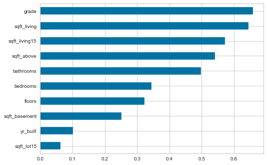
KNN回帰
KNN回帰は距離を用いて予測するものです。スケールによって距離を測るのが難しくなるので、標準化した変数を用いて予測します。
X_scaled = scale(X)フィッティング
model = KNeighborsRegressor()
model.fit(X=X_scaled, y=y)
予測
y_pred = model.predict(X_scaled)回帰モデル誤差評価
from sklearn.metrics import (mean_squared_error,
                            mean_absolute_error,
                            mean_squared_log_error,
                            median_absolute_error,
                            explained_variance_score,
                            r2_score)
予測誤差を計算する
誤差は真の値からの偏差ですが、残差は推定値(たとえば、母平均の推定値)からの偏差です。
error = (y - y_pred).rename('Prediction Errors')scores = dict(
rmse=np.sqrt(mean_squared_error(y_true=y, y_pred=y_pred)),
rmsle=np.sqrt(mean_squared_log_error(y_true=y, y_pred=y_pred)),
mean_ae=mean_absolute_error(y_true=y, y_pred=y_pred),
median_ae=median_absolute_error(y_true=y, y_pred=y_pred),
r2score=explained_variance_score(y_true=y, y_pred=y_pred)
)fig, axes = plt.subplots(ncols=3, figsize=(15, 4))
sns.scatterplot(x=y, y=y_pred, ax=axes[0])
axes[0].set_xlabel('Log Price')
axes[0].set_ylabel('Predictions')
axes[0].set_ylim(11, 16)
axes[0].set_title('Predicted vs. Actuals')
sns.distplot(error, ax=axes[1])
axes[1].set_title('Residuals')
pd.Series(scores).plot.barh(ax=axes[2], title='Error Metrics')
fig.suptitle('In-Sample Regression Errors', fontsize=16)
sns.despine()
fig.tight_layout()
fig.subplots_adjust(top=.88)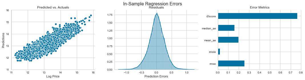
交差検定
ここでは、ハイパーパラメータチューニングを行う。モデルのパラメータを最適化します。今回はRMSEという二乗誤差を最小化するように最適化します。
def rmse(y_true, pred):
   return np.sqrt(mean_squared_error(y_true=y_true, y_pred=pred))

rmse_score = make_scorer(rmse)
cv_rmse = {}
n_neighbors = [1] + list(range(5, 51, 5))
for n in n_neighbors:
pipe = Pipeline([('scaler', StandardScaler()),
('knn', KNeighborsRegressor(n_neighbors=n))])
cv_rmse[n] = cross_val_score(pipe,
X=X,
y=y,
scoring=rmse_score,
cv=5)cv_rmse = pd.DataFrame.from_dict(cv_rmse, orient='index')
best_n, best_rmse = cv_rmse.mean(1).idxmin(), cv_rmse.mean(1).min()
cv_rmse = cv_rmse.stack().reset_index()
cv_rmse.columns =['n', 'fold', 'RMSE']試行回数と誤差の推移について見ていきます。
ax = sns.lineplot(x='n', y='RMSE', data=cv_rmse)
ax.set_title(f'Cross-Validation Results KNN | Best N: {best_n:d} | Best RMSE: {best_rmse:.2f}');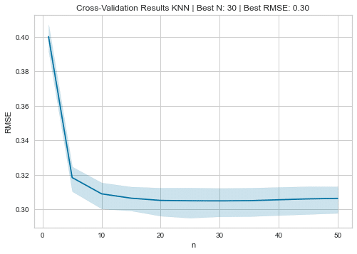
観測値 vs 予測値
pipe = Pipeline([('scaler', StandardScaler()),
                ('knn', KNeighborsRegressor(n_neighbors=best_n))])
y_pred = cross_val_predict(pipe, X, y, cv=5)

ax = sns.scatterplot(x=y, y=y_pred)
y_range = list(range(int(y.min() + 1), int(y.max() + 1)))
pd.Series(y_range, index=y_range).plot(ax=ax, lw=2, c='darkred');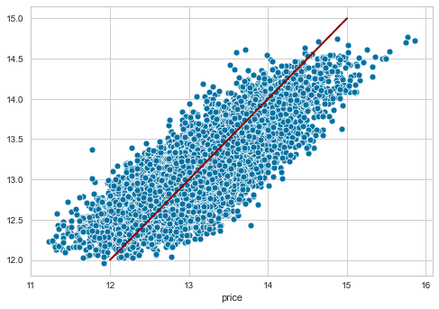
交差検定の誤差
error = (y - y_pred).rename('Prediction Errors')scores = dict(
rmse=np.sqrt(mean_squared_error(y_true=y, y_pred=y_pred)),
rmsle=np.sqrt(mean_squared_log_error(y_true=y, y_pred=y_pred)),
mean_ae=mean_absolute_error(y_true=y, y_pred=y_pred),
median_ae=median_absolute_error(y_true=y, y_pred=y_pred),
r2score=explained_variance_score(y_true=y, y_pred=y_pred)
)fig, axes = plt.subplots(ncols=3, figsize=(15, 5))
sns.scatterplot(x=y, y=y_pred, ax=axes[0])
axes[0].set_xlabel('Log Price')
axes[0].set_ylabel('Predictions')
axes[0].set_ylim(11, 16)
sns.distplot(error, ax=axes[1])
pd.Series(scores).plot.barh(ax=axes[2], title='Error Metrics')
fig.suptitle('Cross-Validation Regression Errors', fontsize=24)
fig.tight_layout()
plt.subplots_adjust(top=.8);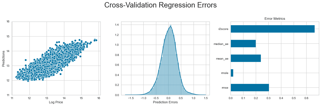
グリッドサーチCV
詳細はsklearnを確認。ここもパラメーターチューニングになります。
pipe = Pipeline([('scaler', StandardScaler()),
                ('knn', KNeighborsRegressor())])

n_folds = 5
n_neighbors = tuple(range(5, 101, 5))

param_grid = {'knn__n_neighbors': n_neighbors}

estimator = GridSearchCV(estimator=pipe,
                        param_grid=param_grid,
                        cv=n_folds,
                        scoring=rmse_score,
#                          n_jobs=-1
                       )
estimator.fit(X=X, y=y)

'''
GridSearchCV(cv=5,
            estimator=Pipeline(steps=[('scaler', StandardScaler()),
                                      ('knn', KNeighborsRegressor())]),
            param_grid={'knn__n_neighbors': (5, 10, 15, 20, 25, 30, 35, 40, 45,
                                             50, 55, 60, 65, 70, 75, 80, 85,
                                             90, 95, 100)},
            scoring=make_scorer(rmse))
'''
cv_results = estimator.cv_results_test_scores = pd.DataFrame({fold: cv_results[f'split{fold}_test_score'] for fold in range(n_folds)},
index=n_neighbors).stack().reset_index()
test_scores.columns = ['k', 'fold', 'RMSE']mean_rmse = test_scores.groupby('k').RMSE.mean()
best_k, best_score = mean_rmse.idxmin(), mean_rmse.min()sns.pointplot(x='k', y='RMSE', data=test_scores, scale=.3, join=False, errwidth=2)
plt.title('Cross Validation Results')
sns.despine()
plt.tight_layout()
plt.gcf().set_size_inches(10, 5);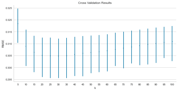
訓練と評価カーブをyellowbricksで見る。
yellowbricksとは機械学習の視覚化のためのツールです。こちらをご参照ください。学習曲線についてはこちら。
fig, ax = plt.subplots(figsize=(16, 9))
val_curve = ValidationCurve(KNeighborsRegressor(),
                     param_name='n_neighbors',
                     param_range=n_neighbors,
                     cv=5,
                     scoring=rmse_score,
#                       n_jobs=-1,
                     ax=ax)
val_curve.fit(X, y)
val_curve.poof()
sns.despine()
fig.tight_layout();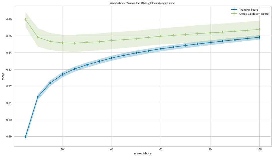
二値分類
y_binary = (y>y.median()).astype(int)n_neighbors = tuple(range(5, 151, 10))
n_folds = 5
scoring = 'roc_auc'pipe = Pipeline([('scaler', StandardScaler()),
('knn', KNeighborsClassifier())])
param_grid = {'knn__n_neighbors': n_neighbors}
estimator = GridSearchCV(estimator=pipe,
param_grid=param_grid,
cv=n_folds,
scoring=scoring,
# n_jobs=-1
)
estimator.fit(X=X, y=y_binary)
'''
GridSearchCV(cv=5,
estimator=Pipeline(steps=[('scaler', StandardScaler()),
('knn', KNeighborsClassifier())]),
param_grid={'knn__n_neighbors': (5, 15, 25, 35, 45, 55, 65, 75, 85,
95, 105, 115, 125, 135, 145)},
scoring='roc_auc')
'''best_k = estimator.best_params_['knn__n_neighbors']fig, ax = plt.subplots(figsize=(16, 9))
val_curve = ValidationCurve(KNeighborsClassifier(),
param_name='n_neighbors',
param_range=n_neighbors,
cv=n_folds,
scoring=scoring,
# n_jobs=-1,
ax=ax)
val_curve.fit(X, y_binary)
val_curve.poof()
sns.despine()
fig.tight_layout();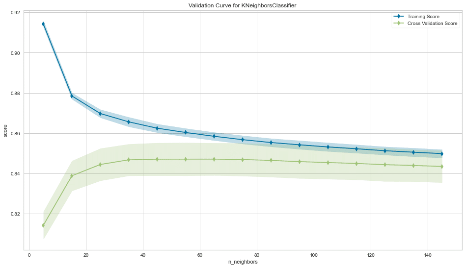
fig, ax = plt.subplots(figsize=(16, 9))
l_curve = LearningCurve(KNeighborsClassifier(n_neighbors=best_k),
                       train_sizes=np.arange(.1, 1.01, .1),
                       scoring=scoring,
                       cv=5,
#                         n_jobs=-1,
                       ax=ax)
l_curve.fit(X, y_binary)
l_curve.poof()
sns.despine()
fig.tight_layout();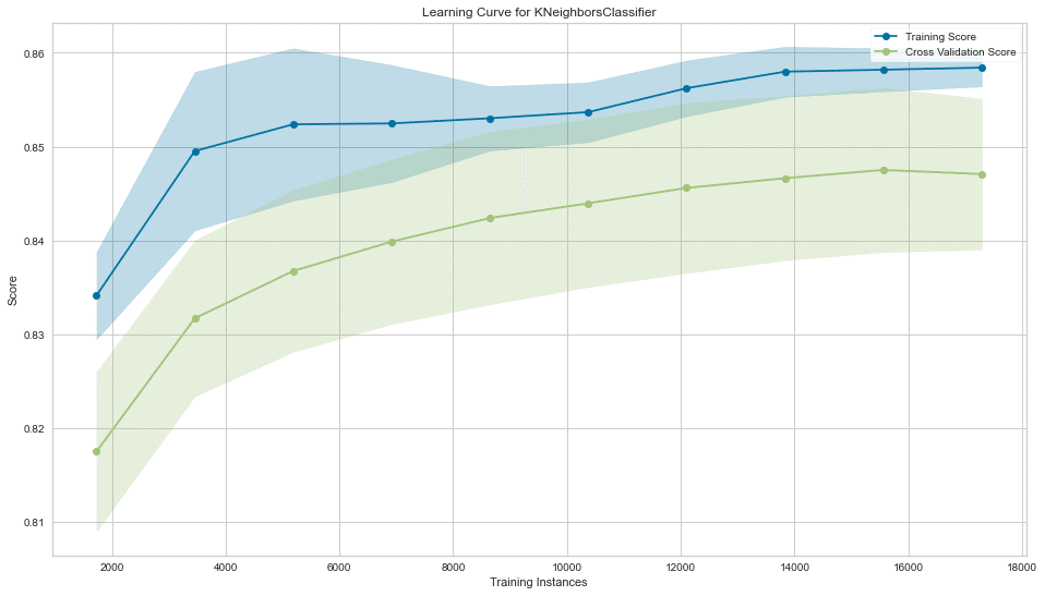
分類の評価関数一覧
from sklearn.metrics import (classification_report,
                            accuracy_score,
                            zero_one_loss,
                            roc_auc_score,
                            roc_curve,
                            brier_score_loss,
                            cohen_kappa_score,
                            confusion_matrix,
                            fbeta_score,
                            hamming_loss,
                            hinge_loss,
                            jaccard_score,
                            log_loss,
                            matthews_corrcoef,
                            f1_score,
                            average_precision_score,
                            precision_recall_curve)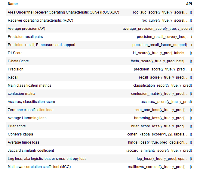
y_score = cross_val_predict(KNeighborsClassifier(best_k),
                          X=X,
                          y=y_binary,
                          cv=5,
                          n_jobs=-1,
                          method='predict_proba')[:, 1]
評価するために予測値と予測確率を用いる。
pred_scores = dict(y_true=y_binary,y_score=y_score)ROC AUC
roc_auc_score(**pred_scores)cols = ['False Positive Rate', 'True Positive Rate', 'threshold']
roc = pd.DataFrame(dict(zip(cols, roc_curve(**pred_scores))))Precision Recall
precision, recall, ts = precision_recall_curve(y_true=y_binary, probas_pred=y_score)
pr_curve = pd.DataFrame({'Precision': precision, 'Recall': recall})
F1スコア
f1 = pd.Series({t: f1_score(y_true=y_binary, y_pred=y_score>t) for t in ts})
best_threshold = f1.idxmax()
二値分類評価結果プロット
fig, axes = plt.subplots(ncols=3, figsize=(15, 5))

ax = sns.scatterplot(x='False Positive Rate', y='True Positive Rate', data=roc, size=5, legend=False, ax=axes[0])
axes[0].plot(np.linspace(0,1,100), np.linspace(0,1,100), color='k', ls='--', lw=1)
axes[0].fill_between(y1=roc['True Positive Rate'], x=roc['False Positive Rate'], alpha=.5,color='darkred')
axes[0].set_title('Receiver Operating Characteristic')


sns.scatterplot(x='Recall', y='Precision', data=pr_curve, ax=axes[1])
axes[1].set_ylim(0,1)
axes[1].set_title('Precision-Recall Curve')


f1.plot(ax=axes[2], title='F1 Scores', ylim=(0,1))
axes[2].set_xlabel('Threshold')
axes[2].axvline(best_threshold, lw=1, ls='--', color='k')
axes[2].text(text=f'Max F1 @ {best_threshold:.2f}', x=.75, y=.95, s=5)
sns.despine()
fig.tight_layout();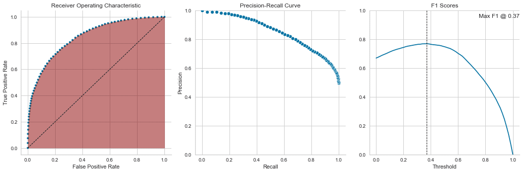
平均precision
average_precision_score(y_true=y_binary, y_score=y_score)バリアスコア
brier_score_loss(y_true=y_binary, y_prob=y_score)混合行列
confusion_matrix(**scores)正答率(Accuracy)
accuracy_score(**scores)ゼローワン 損失 (Zero-One loss)
zero_one_loss(**scores)ハミング損失 (Hamming loss)
不正解だったラベルの比
hamming_loss(**scores)カッパ係数(Cohen's Kappa)
カッパ係数とは、二つの評価のカテゴリ評価の一致度を見るためにある。
cohen_kappa_score(y1=y_binary, y2=y_pred)ヒンジ損失 (Hinge Loss)
hinge_loss(y_true=y_binary, pred_decision=y_pred)ジャカール指数 (Jaccard Similarity)
jaccard_score(**scores)対数損失/交差エントロピー損失
log_loss(**scores)マシューズ相関係数
matthews_corrcoef(**scores)多クラス分類
y_multi = pd.qcut(y, q=3, labels=[0,1,2])n_neighbors = tuple(range(5, 151, 10))
n_folds = 5
scoring = 'accuracy'pipe = Pipeline([('scaler', StandardScaler()),
('knn', KNeighborsClassifier())])
param_grid = {'knn__n_neighbors': n_neighbors}
estimator = GridSearchCV(estimator=pipe,
param_grid=param_grid,
cv=n_folds,
n_jobs=-1
)
estimator.fit(X=X, y=y_multi)
'''
GridSearchCV(cv=5,
estimator=Pipeline(steps=[('scaler', StandardScaler()),
('knn', KNeighborsClassifier())]),
n_jobs=-1,
param_grid={'knn__n_neighbors': (5, 15, 25, 35, 45, 55, 65, 75, 85,
95, 105, 115, 125, 135, 145)})
'''y_pred = cross_val_predict(estimator.best_estimator_,
X=X,
y=y_multi,
cv=5,
n_jobs=-1,
method='predict')print(classification_report(y_true=y_multi, y_pred=y_pred))
'''
precision recall f1-score support
0 0.67 0.71 0.69 7226
1 0.52 0.52 0.52 7223
2 0.77 0.74 0.75 7164
accuracy 0.65 21613
macro avg 0.65 0.65 0.65 21613
weighted avg 0.65 0.65 0.65 21613
'''まとめ
今回は機械学習の予測の種類とパラメーターチューニング方法、評価方法について説明した。
この記事が気に入ったらサポートをしてみませんか?