第7章 線形モデル編: 第5節 線形回帰で株価予測をする

はじめに
本記事では、線形回帰モデルとリッジ回帰とラッソ回帰から交差検定を用いて予測モデルを作成します。予測モデルの結果を評価し、最後に3つのモデルを比較したいと思います。
リッジ回帰とラッソ回帰についてはこちらの記事が分かりやすいです。
インポートと設定
import warnings
warnings.filterwarnings('ignore')
%matplotlib inline
from time import time
from pathlib import Path
import pandas as pd
import numpy as np
from scipy.stats import spearmanr
from sklearn.metrics import mean_squared_error
from sklearn.preprocessing import StandardScaler
from sklearn.linear_model import LinearRegression, Ridge, Lasso
from sklearn.pipeline import Pipeline
import seaborn as sns
import matplotlib.pyplot as plt
from matplotlib.ticker import FuncFormattersns.set_style('darkgrid')
idx = pd.IndexSliceYEAR = 252データの読み込み
with pd.HDFStore('data.h5') as store:
   data = (store['model_data']
           .dropna()
           .drop(['open', 'close', 'low', 'high'], axis=1))
data.index.names = ['symbol', 'date']data = data.drop([c for c in data.columns if 'lag' in c], axis=1)フィルタリング
data = data[data.dollar_vol_rank<100]目的変数と説明変数の定義
y = data.filter(like='target')
X = data.drop(y.columns, axis=1)
X = X.drop(['dollar_vol', 'dollar_vol_rank', 'volume', 'consumer_durables'], axis=1)ここまでは前回と同じですので、そちらも参考にしてくださいませ。
カスタムマルチ時系列交差検定
こちらのカスタムマルチ時系列交差検定について解説します。
例えば、2週間訓練して2週間テストして、それを2週間ずつズラしたいと思います。いわゆるウォークフォワード法っていう手法になります。しかも、こちらの良い所は、テスト期間の初めはデータが漏れる可能性があり(フォワードリターンの期間によって)、それでデータを一部取り除く作業もしております。
class MultipleTimeSeriesCV:
   """Generates tuples of train_idx, test_idx pairs
   Assumes the MultiIndex contains levels 'symbol' and 'date'
   purges overlapping outcomes"""

   def __init__(self,
                n_splits=3,
                train_period_length=126,
                test_period_length=21,
                lookahead=None,
                shuffle=False):
       self.n_splits = n_splits
       self.lookahead = lookahead
       self.test_length = test_period_length
       self.train_length = train_period_length
       self.shuffle = shuffle

   def split(self, X, y=None, groups=None):
       unique_dates = X.index.get_level_values('date').unique()
       days = sorted(unique_dates, reverse=True)

       split_idx = []
       for i in range(self.n_splits):
           test_end_idx = i * self.test_length
           test_start_idx = test_end_idx + self.test_length
           train_end_idx = test_start_idx + + self.lookahead - 1
           train_start_idx = train_end_idx + self.train_length + self.lookahead - 1
           split_idx.append([train_start_idx, train_end_idx,
                             test_start_idx, test_end_idx])

       dates = X.reset_index()[['date']]
       for train_start, train_end, test_start, test_end in split_idx:
           train_idx = dates[(dates.date > days[train_start])
                             & (dates.date <= days[train_end])].index
           test_idx = dates[(dates.date > days[test_start])
                            & (dates.date <= days[test_end])].index
           if self.shuffle:
               np.random.shuffle(list(train_idx))
           yield train_idx, test_idx

   def get_n_splits(self, X, y, groups=None):
       return self.n_splits
出力例
train_period_length = 63
test_period_length = 10
n_splits = int(3 * YEAR/test_period_length)
lookahead =1

cv = MultipleTimeSeriesCV(n_splits=n_splits,
                         test_period_length=test_period_length,
                         lookahead=lookahead,
                         train_period_length=train_period_length)
i = 0
for train_idx, test_idx in cv.split(X=data):
train = data.iloc[train_idx]
train_dates = train.index.get_level_values('date')
test = data.iloc[test_idx]
test_dates = test.index.get_level_values('date')
df = train.reset_index().append(test.reset_index())
n = len(df)
assert n== len(df.drop_duplicates())
print(train.groupby(level='symbol').size().value_counts().index[0],
train_dates.min().date(), train_dates.max().date(),
test.groupby(level='symbol').size().value_counts().index[0],
test_dates.min().date(), test_dates.max().date())
i += 1
if i == 10:
break
'''
63 2017-08-16 2017-11-14 10 2017-11-15 2017-11-29
63 2017-08-02 2017-10-30 10 2017-10-31 2017-11-14
63 2017-07-19 2017-10-16 10 2017-10-17 2017-10-30
63 2017-07-05 2017-10-02 10 2017-10-03 2017-10-16
63 2017-06-20 2017-09-18 10 2017-09-19 2017-10-02
63 2017-06-06 2017-09-01 10 2017-09-05 2017-09-18
63 2017-05-22 2017-08-18 10 2017-08-21 2017-09-01
63 2017-05-08 2017-08-04 10 2017-08-07 2017-08-18
63 2017-04-24 2017-07-21 10 2017-07-24 2017-08-04
62 2017-04-10 2017-07-07 10 2017-07-10 2017-07-21
'''視覚化ツール
予測値と実際の値の散布図
def plot_preds_scatter(df, ticker=None):
   if ticker is not None:
       idx = pd.IndexSlice
       df = df.loc[idx[ticker, :], :]
   j = sns.jointplot(x='predicted', y='actuals',
                     robust=True, ci=None,
                     line_kws={'lw': 1, 'color': 'k'},
                     scatter_kws={'s': 1},
                     data=df,
                     stat_func=spearmanr,
                     kind='reg')
   j.ax_joint.yaxis.set_major_formatter(
       FuncFormatter(lambda y, _: '{:.1%}'.format(y)))
   j.ax_joint.xaxis.set_major_formatter(
       FuncFormatter(lambda x, _: '{:.1%}'.format(x)))
   j.ax_joint.set_xlabel('Predicted')
   j.ax_joint.set_ylabel('Actuals')
日次情報係数(IC)分布
情報係数定義:
情報係数とは、リターンと投資指標の相関係数です。
def plot_ic_distribution(df, ax=None):
   if ax is not None:
       sns.distplot(df.ic, ax=ax)
   else:
       ax = sns.distplot(df.ic)
   mean, median = df.ic.mean(), df.ic.median()
   ax.axvline(0, lw=1, ls='--', c='k')
   ax.text(x=.05, y=.9,
           s=f'Mean: {mean:8.2f}\nMedian: {median:5.2f}',
           horizontalalignment='left',
           verticalalignment='center',
           transform=ax.transAxes)
   ax.set_xlabel('Information Coefficient')
   sns.despine()
   plt.tight_layout()
ローリング日次IC
def plot_rolling_ic(df):
   fig, axes = plt.subplots(nrows=2, sharex=True, figsize=(14, 8))
   rolling_result = df.sort_index().rolling(21).mean().dropna()
   mean_ic = df.ic.mean()
   rolling_result.ic.plot(ax=axes[0],
                          title=f'Information Coefficient (Mean: {mean_ic:.2f})',
                          lw=1)
   axes[0].axhline(0, lw=.5, ls='-', color='k')
   axes[0].axhline(mean_ic, lw=1, ls='--', color='k')

   mean_rmse = df.rmse.mean()
   rolling_result.rmse.plot(ax=axes[1],
                            title=f'Root Mean Squared Error (Mean: {mean_rmse:.2%})',
                            lw=1,
                            ylim=(0, df.rmse.max()))
   axes[1].axhline(df.rmse.mean(), lw=1, ls='--', color='k')
   sns.despine()
   plt.tight_layout()
sklearnによる線形回帰
交差検定セットアップ
train_period_length = 63
test_period_length = 10
n_splits = int(3 * YEAR / test_period_length)
lookahead = 1

cv = MultipleTimeSeriesCV(n_splits=n_splits,
                         test_period_length=test_period_length,
                         lookahead=lookahead,
                         train_period_length=train_period_length)
線形回帰モデルで交差検定する
%%time
target = f'target_{lookahead}d'
lr_predictions, lr_scores = [], []
lr = LinearRegression()
for i, (train_idx, test_idx) in enumerate(cv.split(X), 1):
   X_train, y_train, = X.iloc[train_idx], y[target].iloc[train_idx]
   X_test, y_test = X.iloc[test_idx], y[target].iloc[test_idx]
   lr.fit(X=X_train, y=y_train)
   y_pred = lr.predict(X_test)

   preds = y_test.to_frame('actuals').assign(predicted=y_pred)
   preds_by_day = preds.groupby(level='date')
   scores = pd.concat([preds_by_day.apply(lambda x: spearmanr(x.predicted,
                                                              x.actuals)[0] * 100)
                       .to_frame('ic'),
                       preds_by_day.apply(lambda x: np.sqrt(mean_squared_error(y_pred=x.predicted,
                                                                               y_true=x.actuals)))
                       .to_frame('rmse')], axis=1)

   lr_scores.append(scores)
   lr_predictions.append(preds)

lr_scores = pd.concat(lr_scores)
lr_predictions = pd.concat(lr_predictions)
'''
CPU times: user 10.6 s, sys: 885 ms, total: 11.5 s
Wall time: 2.94 s
'''
結果の保持
lr_scores.to_hdf('data.h5', 'lr/scores')
lr_predictions.to_hdf('data.h5', 'lr/predictions')
lr_scores = pd.read_hdf('data.h5', 'lr/scores')
lr_predictions = pd.read_hdf('data.h5', 'lr/predictions')評価結果
lr_r, lr_p = spearmanr(lr_predictions.actuals, lr_predictions.predicted)
print(f'Information Coefficient (overall): {lr_r:.3%} (p-value: {lr_p:.4%})')
'''
Information Coefficient (overall): 1.559% (p-value: 0.0022%)
'''
予測 vs 観測 散布図
plot_preds_scatter(lr_predictions)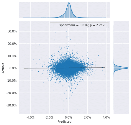
日次IC分布
plot_ic_distribution(lr_scores)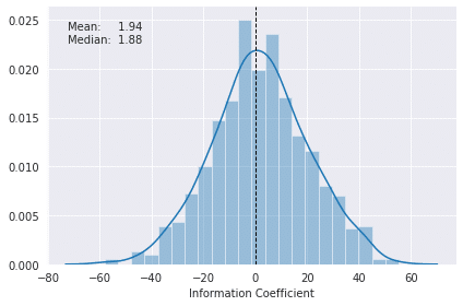
ローリング日次IC
plot_rolling_ic(lr_scores)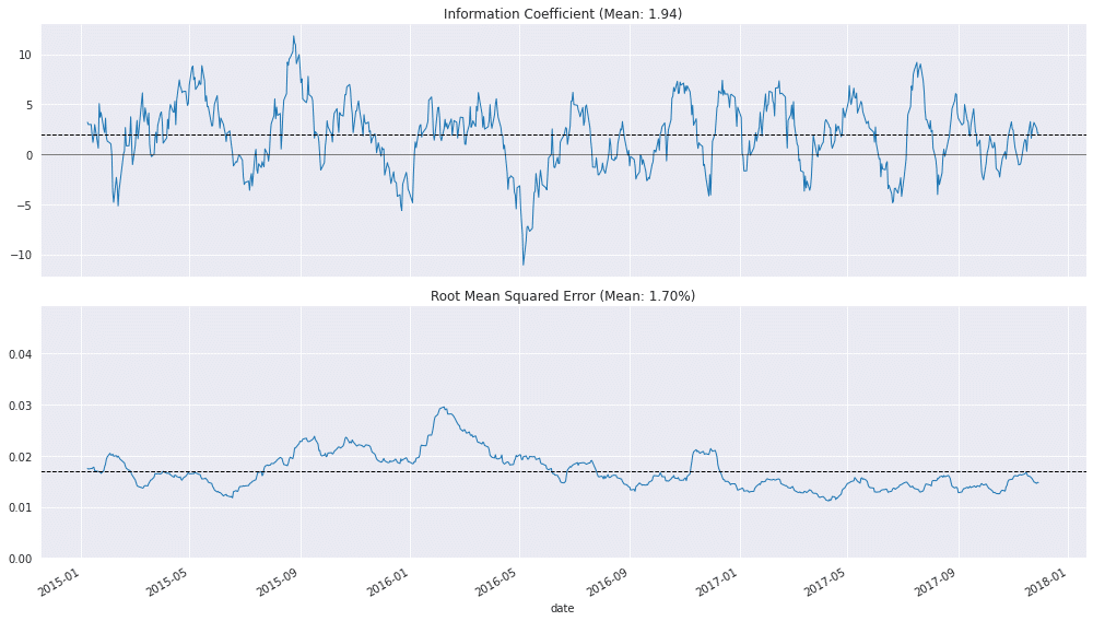
リッジ回帰
ridge_alphas = np.logspace(-4, 4, 9)
ridge_alphas = sorted(list(ridge_alphas) + list(ridge_alphas * 5))
n_splits = int(3 * YEAR/test_period_length)
train_period_length = 63
test_period_length = 10
lookahead = 1
cv = MultipleTimeSeriesCV(n_splits=n_splits,
test_period_length=test_period_length,
lookahead=lookahead,
train_period_length=train_period_length)交差検定を走らせる
target = f'target_{lookahead}d'

X = X.drop([c for c in X.columns if 'year' in c], axis=1)
%%time
ridge_coeffs, ridge_scores, ridge_predictions = {}, [], []
for alpha in ridge_alphas:
print(alpha, end=' ', flush=True)
start = time()
model = Ridge(alpha=alpha,
fit_intercept=False,
random_state=42)
pipe = Pipeline([
('scaler', StandardScaler()),
('model', model)])
coeffs = []
for i, (train_idx, test_idx) in enumerate(cv.split(X), 1):
X_train, y_train, = X.iloc[train_idx], y[target].iloc[train_idx]
X_test, y_test = X.iloc[test_idx], y[target].iloc[test_idx]
pipe.fit(X=X_train, y=y_train)
y_pred = pipe.predict(X_test)
preds = y_test.to_frame('actuals').assign(predicted=y_pred)
preds_by_day = preds.groupby(level='date')
scores = pd.concat([preds_by_day.apply(lambda x: spearmanr(x.predicted,
x.actuals)[0] * 100)
.to_frame('ic'),
preds_by_day.apply(lambda x: np.sqrt(mean_squared_error(y_pred=x.predicted,
y_true=x.actuals)))
.to_frame('rmse')], axis=1)
ridge_scores.append(scores.assign(alpha=alpha))
ridge_predictions.append(preds.assign(alpha=alpha))
coeffs.append(pipe.named_steps['model'].coef_)
ridge_coeffs[alpha] = np.mean(coeffs, axis=0)
print('\n')
'''
0.0001 0.0005 0.001 0.005 0.01 0.05 0.1 0.5 1.0 5.0 10.0 50.0 100.0 500.0 1000.0 5000.0 10000.0 50000.0
CPU times: user 3min 32s, sys: 16.7 s, total: 3min 48s
Wall time: 57.7 s
'''結果の保持
ridge_scores = pd.concat(ridge_scores)
ridge_scores.to_hdf('data.h5', 'ridge/scores')

ridge_coeffs = pd.DataFrame(ridge_coeffs, index=X.columns).T
ridge_coeffs.to_hdf('data.h5', 'ridge/coeffs')

ridge_predictions = pd.concat(ridge_predictions)
ridge_predictions.to_hdf('data.h5', 'ridge/predictions')
ridge_scores = pd.read_hdf('data.h5', 'ridge/scores')
ridge_coeffs = pd.read_hdf('data.h5', 'ridge/coeffs')
ridge_predictions = pd.read_hdf('data.h5', 'ridge/predictions')結果の評価
ridge_r, ridge_p = spearmanr(ridge_predictions.actuals, ridge_predictions.predicted)
print(f'Information Coefficient (overall): {ridge_r:.3%} (p-value: {ridge_p:.4%})')
'''
Information Coefficient (overall): 1.583% (p-value: 0.0000%)
'''
ridge_scores.groupby('alpha').ic.describe()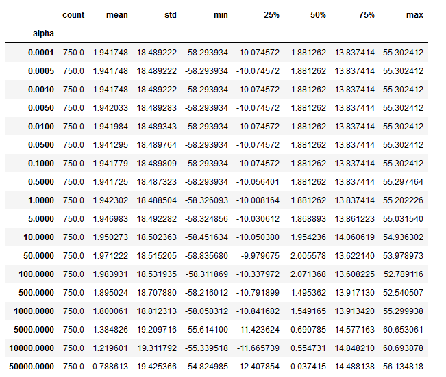
fig, axes = plt.subplots(ncols=2, sharex=True, figsize=(15, 5))

scores_by_alpha = ridge_scores.groupby('alpha').ic.agg(['mean', 'median'])
best_alpha_mean = scores_by_alpha['mean'].idxmax()
best_alpha_median = scores_by_alpha['median'].idxmax()

ax = sns.lineplot(x='alpha',
                 y='ic',
                 data=ridge_scores,
                 estimator=np.mean,
                 label='Mean',
                 ax=axes[0])

scores_by_alpha['median'].plot(logx=True,
                              ax=axes[0],
                              label='Median')

axes[0].axvline(best_alpha_mean,
               ls='--',
               c='k',
               lw=1,
               label='Max. Mean')
axes[0].axvline(best_alpha_median,
               ls='-.',
               c='k',
               lw=1,
               label='Max. Median')
axes[0].legend()
axes[0].set_xscale('log')
axes[0].set_xlabel('Alpha')
axes[0].set_ylabel('Information Coefficient')
axes[0].set_title('Cross Validation Performance')

ridge_coeffs.plot(logx=True,
                 legend=False,
                 ax=axes[1],
                 title='Ridge Coefficient Path')

axes[1].axvline(best_alpha_mean,
               ls='--',
               c='k',
               lw=1,
               label='Max. Mean')
axes[1].axvline(best_alpha_median,
               ls='-.',
               c='k',
               lw=1,
               label='Max. Median')
axes[1].set_xlabel('Alpha')
axes[1].set_ylabel('Coefficient Value')

fig.suptitle('Ridge Results', fontsize=14)
sns.despine()
fig.tight_layout()
fig.subplots_adjust(top=.9)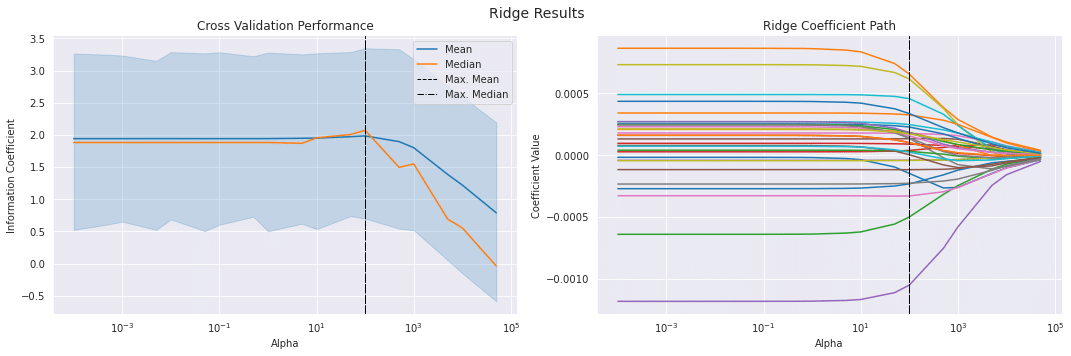
best_alpha = ridge_scores.groupby('alpha').ic.mean().idxmax()
fig, axes = plt.subplots(ncols=2, figsize=(15, 5))
plot_ic_distribution(ridge_scores[ridge_scores.alpha == best_alpha],
                    ax=axes[0])
axes[0].set_title('Daily Information Coefficients')
top_coeffs = ridge_coeffs.loc[best_alpha].abs().sort_values().head(10).index
top_coeffs.tolist()
ridge_coeffs.loc[best_alpha, top_coeffs].sort_values().plot.barh(ax=axes[1],
                                                                title='Top 10 Coefficients')
sns.despine()
fig.tight_layout()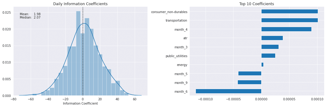
plot_rolling_ic(ridge_scores[ridge_scores.alpha==best_alpha])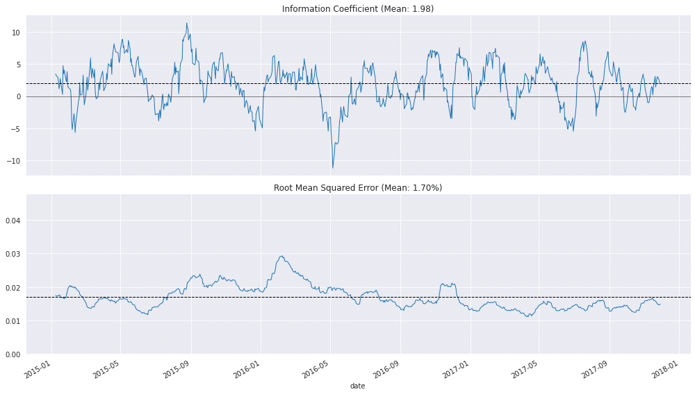
ラッソ交差検定(Lasso CV)
lasso_alphas = np.logspace(-10, -3, 8)train_period_length = 63
test_period_length = 10
YEAR = 252
n_splits = int(3 * YEAR / test_period_length) # three years
lookahead = 1cv = MultipleTimeSeriesCV(n_splits=n_splits,
test_period_length=test_period_length,
lookahead=lookahead,
train_period_length=train_period_length)交差検定する
target = f'target_{lookahead}d'

scaler = StandardScaler()
X = X.drop([c for c in X.columns if 'year' in c], axis=1)
%%time
lasso_coeffs, lasso_scores, lasso_predictions = {}, [], []
for alpha in lasso_alphas:
print(alpha, end=' ', flush=True)
model = Lasso(alpha=alpha,
fit_intercept=False, # StandardScaler centers data
random_state=42,
tol=1e-3,
max_iter=1000,
warm_start=True,
selection='random')
pipe = Pipeline([
('scaler', StandardScaler()),
('model', model)])
coeffs = []
for i, (train_idx, test_idx) in enumerate(cv.split(X), 1):
t = time()
X_train, y_train, = X.iloc[train_idx], y[target].iloc[train_idx]
X_test, y_test = X.iloc[test_idx], y[target].iloc[test_idx]
pipe.fit(X=X_train, y=y_train)
y_pred = pipe.predict(X_test)
preds = y_test.to_frame('actuals').assign(predicted=y_pred)
preds_by_day = preds.groupby(level='date')
scores = pd.concat([preds_by_day.apply(lambda x: spearmanr(x.predicted,
x.actuals)[0] * 100)
.to_frame('ic'),
preds_by_day.apply(lambda x: np.sqrt(mean_squared_error(y_pred=x.predicted,
y_true=x.actuals)))
.to_frame('rmse')],
axis=1)
lasso_scores.append(scores.assign(alpha=alpha))
lasso_predictions.append(preds.assign(alpha=alpha))
coeffs.append(pipe.named_steps['model'].coef_)
lasso_coeffs[alpha] = np.mean(coeffs, axis=0)
'''
1e-10 1e-09 1e-08 1e-07 1e-06 1e-05 0.0001 0.001 CPU times: user 3min 11s, sys: 14.3 s, total: 3min 25s
Wall time: 52.1 s
'''結果の保持
lasso_scores = pd.concat(lasso_scores)
lasso_scores.to_hdf('data.h5', 'lasso/scores')

lasso_coeffs = pd.DataFrame(lasso_coeffs, index=X.columns).T
lasso_coeffs.to_hdf('data.h5', 'lasso/coeffs')

lasso_predictions = pd.concat(lasso_predictions)
lasso_predictions.to_hdf('data.h5', 'lasso/predictions')
結果の評価
best_alpha = lasso_scores.groupby('alpha').ic.mean().idxmax()
preds = lasso_predictions[lasso_predictions.alpha==best_alpha]

lasso_r, lasso_p = spearmanr(preds.actuals, preds.predicted)
print(f'Information Coefficient (overall): {lasso_r:.3%} (p-value: {lasso_p:.4%})')

'''
Information Coefficient (overall): 3.600% (p-value: 0.0000%)
'''lasso_scores.groupby('alpha').ic.agg(['mean', 'median'])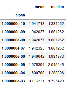
ラッソ係数のパス
fig, axes = plt.subplots(ncols=2, sharex=True, figsize=(15, 5))

scores_by_alpha = lasso_scores.groupby('alpha').ic.agg(['mean', 'median'])
best_alpha_mean = scores_by_alpha['mean'].idxmax()
best_alpha_median = scores_by_alpha['median'].idxmax()

ax = sns.lineplot(x='alpha', y='ic', data=lasso_scores, estimator=np.mean, label='Mean', ax=axes[0])

scores_by_alpha['median'].plot(logx=True, ax=axes[0], label='Median')

axes[0].axvline(best_alpha_mean, ls='--', c='k', lw=1, label='Max. Mean')
axes[0].axvline(best_alpha_median, ls='-.', c='k', lw=1, label='Max. Median')
axes[0].legend()
axes[0].set_xscale('log')
axes[0].set_xlabel('Alpha')
axes[0].set_ylabel('Information Coefficient')
axes[0].set_title('Cross Validation Performance')

lasso_coeffs.plot(logx=True, legend=False, ax=axes[1], title='Lasso Coefficient Path')
axes[1].axvline(best_alpha_mean, ls='--', c='k', lw=1, label='Max. Mean')
axes[1].axvline(best_alpha_median, ls='-.', c='k', lw=1, label='Max. Median')
axes[1].set_xlabel('Alpha')
axes[1].set_ylabel('Coefficient Value')

fig.suptitle('Lasso Results', fontsize=14)
fig.tight_layout()
fig.subplots_adjust(top=.9)
sns.despine();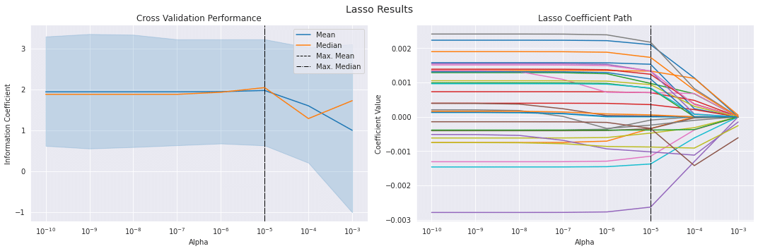
ラッソIC分布と上位10特徴量
best_alpha = lasso_scores.groupby('alpha').ic.mean().idxmax()

fig, axes = plt.subplots(ncols=2, figsize=(15, 5))
plot_ic_distribution(lasso_scores[lasso_scores.alpha==best_alpha], ax=axes[0])
axes[0].set_title('Daily Information Coefficients')

top_coeffs = lasso_coeffs.loc[best_alpha].abs().sort_values().head(10).index
top_coeffs.tolist()
lasso_coeffs.loc[best_alpha, top_coeffs].sort_values().plot.barh(ax=axes[1], title='Top 10 Coefficients')

sns.despine()
fig.tight_layout();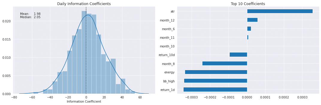
結果の比較
best_ridge_alpha = ridge_scores.groupby('alpha').ic.mean().idxmax()
best_ridge_preds = ridge_predictions[ridge_predictions.alpha==best_ridge_alpha]
best_ridge_scores = ridge_scores[ridge_scores.alpha==best_ridge_alpha]
best_lasso_alpha = lasso_scores.groupby('alpha').ic.mean().idxmax()
best_lasso_preds = lasso_predictions[lasso_predictions.alpha==best_lasso_alpha]
best_lasso_scores = lasso_scores[lasso_scores.alpha==best_lasso_alpha]df = pd.concat([lr_scores.assign(Model='Linear Regression'),
best_ridge_scores.assign(Model='Ridge Regression'),
best_lasso_scores.assign(Model='Lasso Regression')]).drop('alpha', axis=1)
df.columns = ['IC', 'RMSE', 'Model']scores = df.groupby('Model').IC.agg(['mean', 'median'])
fig, axes = plt.subplots(ncols=2, figsize=(14,4), sharey=True, sharex=True)
scores['mean'].plot.barh(ax=axes[0], xlim=(1.85, 2), title='Mean')
scores['median'].plot.barh(ax=axes[1], xlim=(1.8, 2.1), title='Median')
axes[0].set_xlabel('Daily IC')
axes[1].set_xlabel('Daily IC')
fig.suptitle('Daily Information Coefficient by Model', fontsize=14)
sns.despine()
fig.tight_layout()
fig.subplots_adjust(top=.9)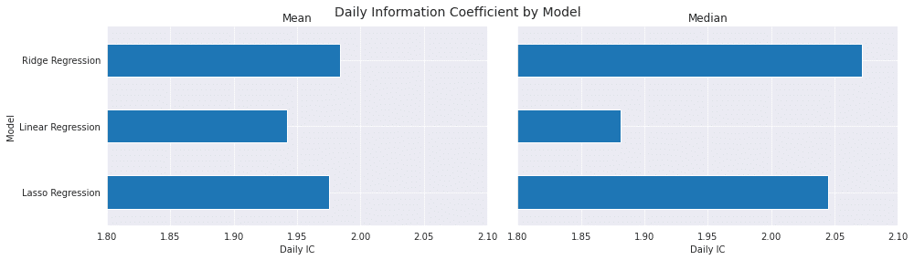
結果は線形回帰モデルよりもリッジ回帰の方が圧倒的に良いですね(*'ω'*)
本記事のコードはそのまま使えますので、リッジ回帰のやり方はご参考にしてくださいませ(*'ω'*)
この記事が気に入ったらサポートをしてみませんか?