
第10章:ベイジアンML-ダイナミックSR 第2節: PyMC3ワークフロー

はじめに
本チャプターではPyMC3を使用しますので、使用方法について解説していきます。
githubはこちらをご参照ください。
PyMC3とは?
PyMC3は、ベイズ統計モデリングと確率的機械学習のためのPythonパッケージで、高度なマルコフ連鎖モンテカルロ(MCMC)アルゴリズムと変分推論(VI)アルゴリズムに焦点を当てています。その柔軟性と拡張性により、様々な問題に適用できます。
インポートと設定
import warnings
warnings.filterwarnings('ignore')
%matplotlib inline
from pathlib import Path
import pickle
import pandas as pd
import numpy as np
from scipy import stats
import pandas_datareader.data as web
from sklearn.preprocessing import scale
from sklearn.model_selection import train_test_split
from sklearn.feature_selection import mutual_info_classif
from sklearn.metrics import roc_auc_score
import theano
import pymc3 as pm
from pymc3.variational.callbacks import CheckParametersConvergence
import statsmodels.formula.api as smf
import matplotlib.pyplot as plt
from matplotlib import animation
import seaborn as sns
from IPython.display import HTMLsns.set_style('whitegrid')data_path = Path('data')
fig_path = Path('figures')
model_path = Path('models')
for p in [data_path, fig_path, model_path]:
if not p.exists():
p.mkdir()データセットの準備
ワークフローに集中できるように、小さくてシンプルなデータセットを使用します。連邦準備制度の経済データ(FRED)サービス(第2章を参照)を使用して、米国経済研究所によって定義された米国の不況の日付をダウンロードします。また、景気後退の発生を予測するために一般的に使用される4つの変数(Kelley 2019)を調達し、FREDから利用できます。
4つの変数は以下の通りです。
・10年と3か月間の国債利回りの差として定義される、国債利回り曲線の長期スプレッド。
・ミシガン大学の消費者心理指標
・国家財政状態指数(NFCI)
・NFCI非金融レバレッジサブインデックス
FREDからダウンロード
indicators = ['JHDUSRGDPBR', 'T10Y3M', 'NFCI', 'NFCILEVERAGE', 'UMCSENT']
var_names = ['recession', 'yield_curve', 'financial_conditions', 'leverage', 'sentiment']
features = var_names[1:]
label = var_names[0]var_display = ['Recession', 'Yield Curve', 'Financial Conditions', 'Leverage', 'Sentiment']
col_dict = dict(zip(var_names, var_display))data = (web.DataReader(indicators, 'fred', 1980, 2020)
.ffill()
.resample('M')
.last()
.dropna())
data.columns = var_names全ての特徴量が平均0,標準偏差1になるように標準化します。
data.loc[:, features] = scale(data.loc[:, features])data.info()
'''
<class 'pandas.core.frame.DataFrame'>
DatetimeIndex: 457 entries, 1982-01-31 to 2020-01-31
Freq: M
Data columns (total 5 columns):
# Column Non-Null Count Dtype
--- ------ -------------- -----
0 recession 457 non-null float64
1 yield_curve 457 non-null float64
2 financial_conditions 457 non-null float64
3 leverage 457 non-null float64
4 sentiment 457 non-null float64
dtypes: float64(5)
memory usage: 21.4 KB
'''データ探索
まず全特徴量の相互情報量を見ていきます。相互情報量のチャプターは第6章 機械学習プロセス編: 第二節 情報理論と利用して特徴量を分析するで解説しています。
mi = []
months = list(range(1, 25))
for month in months:
   df_ = data.copy()
   df_[label] = df_[label].shift(-month)
   df_ = df_.dropna()
   mi.append(mutual_info_classif(df_.loc[:, features], df_[label]))
mi = pd.DataFrame(mi, columns=features, index=months)mi.sum(1).mul(100).iloc[:12].sort_index(ascending=False).plot.barh(figsize=(12, 4), xlim=(15, 40));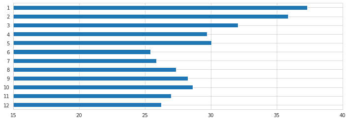
fig, ax = plt.subplots(figsize=(20, 3))
sns.heatmap(mi.rename(columns=col_dict).T*100, cmap='Greys', ax=ax, annot=True, fmt='.1f', cbar=False)
ax.set_xlabel('Lead Time (Months)')
ax.set_title('Mutual Information between Indicators and Recession by Lead Time')
fig.tight_layout();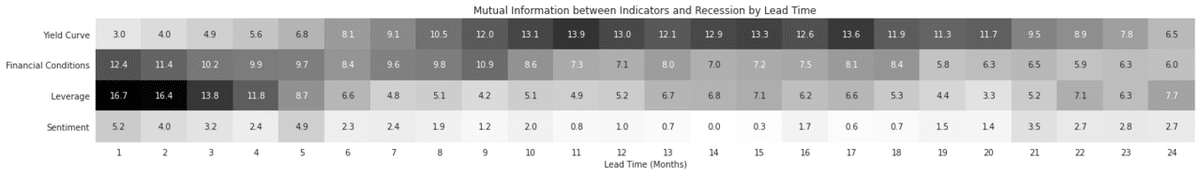
data[label] = data[label].shift(-12)
data = data.dropna()
data_ = pd.melt(data.rename(columns=col_dict), id_vars='Recession').rename(columns=str.capitalize)
g = sns.catplot(x='Recession', y='Value', col='Variable', data=data_, kind='box');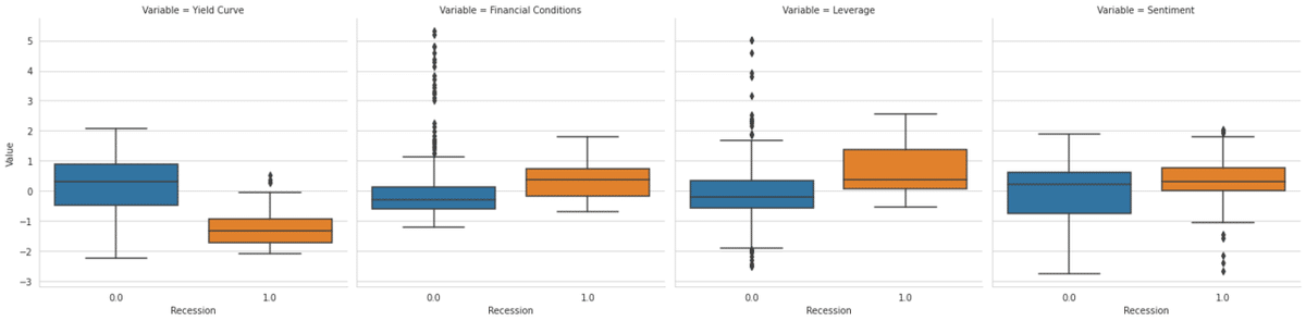
X = data.loc[:, features]
y = data[label]
y.value_counts()
'''
0.0 393
1.0 52
Name: recession, dtype: int64
'''data.to_csv('data/recessions.csv')ディスクから読み込む
data = pd.read_csv('data/recessions.csv', index_col=0)
data.info()
'''
<class 'pandas.core.frame.DataFrame'>
Index: 445 entries, 1982-01-31 to 2019-01-31
Data columns (total 5 columns):
#   Column                Non-Null Count  Dtype
---  ------                --------------  -----
0   recession             445 non-null    float64
1   yield_curve           445 non-null    float64
2   financial_conditions  445 non-null    float64
3   leverage              445 non-null    float64
4   sentiment             445 non-null    float64
dtypes: float64(5)
memory usage: 20.9+ KB
'''
モデル
simple_model = 'recession ~ yield_curve + leverage'
full_model =  simple_model + ' + financial_conditions + sentiment'
MAP推定
確率的プログラム(probabilistic programming)は、観測された確率変数と観測されていない確率変数(RVs : random variables)で構成されます。説明したように、尤度分布を介して観測されたRVと、事前分布を介して観測されなかったRVを定義します。 PyMC3には、この目的のための多数の確率分布が含まれています。
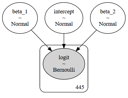
PyMC3ライブラリを使用すると、ロジスティック回帰の近似ベイズ推定を簡単に実行できます。ロジスティック回帰は、次の図に概要を示すように、個人iがk個の特徴に基づいて高収入を得る確率をモデル化します。
マニュアルモデル仕様
context managerを使用して、後で確率モデルとして参照できるmanual_logistic_modelを定義します。
・切片と2つの特徴の観測されていないパラメーターの確率変数は、平均0と標準偏差100の正規分布を仮定する情報のない事前分布を使用して表されます。
・尤度は、ロジスティック回帰の仕様に従ってパラメーターをデータと組み合わせます
・結果は、可能性によって与えられる成功確率を持つベルヌーイRVとしてモデル化されます。
with pm.Model() as manual_logistic_model:
   # random variables for coefficients with
   # uninformative priors for each parameter

   intercept = pm.Normal('intercept', 0, sd=100)
   beta_1 = pm.Normal('beta_1', 0, sd=100)
   beta_2 = pm.Normal('beta_2', 0, sd=100)

   # Transform random variables into vector of probabilities p(y_i=1)
   # according to logistic regression model specification.
   likelihood = pm.invlogit(intercept +
                            beta_1 * data.yield_curve +
                            beta_2 * data.leverage)

   # Bernoulli random vector with probability of success
   # given by sigmoid function and actual data as observed
   pm.Bernoulli(name='logit',
                p=likelihood,
observed=data.recession)manual_logistic_model.model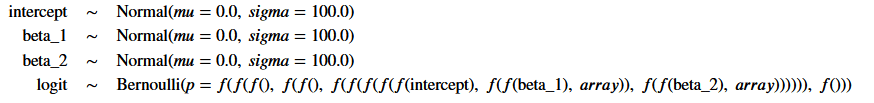
コマンドpm.model_to_graphviz(manual_logistic_model)は、下に表示されるプレート表記を生成します。
観測されていないパラメータは明るいものとして、観測された要素は暗い円として表示されます。四角形は、モデル定義に含まれるデータによって暗示される、観測されたモデル要素の繰り返し数を示します。
推定を実行する
with manual_logistic_model:
   # compute maximum a-posteriori estimate
   # for logistic regression weights
   manual_map_estimate = pm.find_MAP()
def print_map(result):
return pd.Series({k: np.asscalar(v) for k, v in result.items()})print_map(manual_map_estimate)
'''
intercept -4.491536
beta_1 -2.856696
beta_2 1.373219
dtype: float64
'''一般化線形モデル(GLM)
PyMC3には多数の一般的なモデルが含まれているため、通常はカスタムアプリケーションの手動仕様をそのまま使用できます。
次のコードは、統計言語Rに着想を得てpatsyライブラリによってpythonに移植された数式形式を使用して、一般化線形モデル(GLM)ファミリーのメンバーと同じロジスティック回帰を定義します。
with pm.Model() as logistic_model:
   pm.glm.GLM.from_formula(simple_model,
                           data,
family=pm.glm.families.Binomial())pm.model_to_graphviz(logistic_model)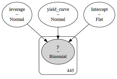
MAP推定
定義したばかりのモデルの.find_MAPメソッドを使用して、3つのパラメーターのポイントMAP推定を取得します。
with logistic_model:
map_estimate = pm.find_MAP()PyMC3は、quasi-Newton Broyden-Fletcher-Goldfarb-Shanno (BFGS) アルゴリズムを使用して最高密度の事後点(posterior point)を見つけるという最適化問題を解決します。scipyライブラリによって提供されるいくつかの代替案も提供します。結果は、対応するstatsmodels推定と実質的に同じです。
model = smf.logit(formula=simple_model, data=data)
result = model.fit()
print(result.summary())
'''
Optimization terminated successfully.
        Current function value: 0.187081
        Iterations 9
                          Logit Regression Results
==============================================================================
Dep. Variable:              recession   No. Observations:                  445
Model:                          Logit   Df Residuals:                      442
Method:                           MLE   Df Model:                            2
Date:                Thu, 13 Aug 2020   Pseudo R-squ.:                  0.4812
Time:                        06:55:48   Log-Likelihood:                -83.251
converged:                       True   LL-Null:                       -160.47
Covariance Type:            nonrobust   LLR p-value:                 2.909e-34
===============================================================================
                 coef    std err          z      P>|z|      [0.025      0.975]
-------------------------------------------------------------------------------
Intercept      -4.4917      0.532     -8.439      0.000      -5.535      -3.448
yield_curve    -2.8568      0.383     -7.458      0.000      -3.608      -2.106
leverage        1.3733      0.235      5.833      0.000       0.912       1.835
===============================================================================
'''
print_map(map_estimate)
'''
Intercept -4.491728
yield_curve -2.856829
leverage 1.373285
dtype: float64
'''result.params
'''
Intercept -4.491692
yield_curve -2.856796
leverage 1.373268
dtype: float64
'''マルコフ連鎖モンテカルロ
def plot_traces(traces, burnin=2000):
   summary = pm.summary(traces[burnin:])['mean'].to_dict()
   ax = pm.traceplot(traces[burnin:],
                     figsize=(15, len(traces.varnames)*1.5),
                     lines=summary)

   for i, mn in enumerate(summary.values()):
       ax[i, 0].annotate(f'{mn:.2f}', xy=(mn, 0),
                         xycoords='data', xytext=(5, 10),
                         textcoords='offset points',
                         rotation=90, va='bottom',
                         fontsize='large',
                         color='#AA0022')
モデルの定義
完全なモデルを使用して、マルコフ連鎖モンテカルロ推論を説明します。
with pm.Model() as logistic_model:
   pm.glm.GLM.from_formula(formula=full_model,
                           data=data,
                           family=pm.glm.families.Binomial())
logistic_model.basic_RVs
'''
[Intercept, yield_curve, leverage, financial_conditions, sentiment, y]
'''メトロポリス・ヘイスティングス法
Metropolis-Hastingsアルゴリズムを使用して、事後分布からサンプリングします。
収束を高速化するための提案分布の分散などのMetropolis-Hastingsのハイパーパラメーターを調べます。関数plot_tracesを使用して、収束を視覚的に検査します。
MAP-estimateを使用してサンプリングスキームを初期化し、処理速度を上げることもできます。これは、可能性のあるポイントから開始するため、ウォームアップ(burnin)期間が短くなります。
with logistic_model:
   trace_mh = pm.sample(tune=1000,
                        draws=5000,
                        step=pm.Metropolis(),
                        cores=4)
'''
Multiprocess sampling (4 chains in 4 jobs)
CompoundStep
>Metropolis: [sentiment]
>Metropolis: [financial_conditions]
>Metropolis: [leverage]
>Metropolis: [yield_curve]
>Metropolis: [Intercept]
'''
経過の調査
plot_traces(trace_mh, burnin=0)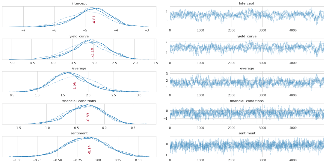
pm.trace_to_dataframe(trace_mh).info()
'''
<class 'pandas.core.frame.DataFrame'>
RangeIndex: 20000 entries, 0 to 19999
Data columns (total 5 columns):
#   Column                Non-Null Count  Dtype
---  ------                --------------  -----
0   Intercept             20000 non-null  float64
1   yield_curve           20000 non-null  float64
2   leverage              20000 non-null  float64
3   financial_conditions  20000 non-null  float64
4   sentiment             20000 non-null  float64
dtypes: float64(5)
memory usage: 781.4 KB
'''
訓練を続ける
with logistic_model:
   trace_mh = pm.sample(draws=100000,
                        step=pm.Metropolis(),
                        trace=trace_mh)
'''
Multiprocess sampling (2 chains in 2 jobs)
CompoundStep
>Metropolis: [sentiment]
>Metropolis: [financial_conditions]
>Metropolis: [leverage]
>Metropolis: [yield_curve]
>Metropolis: [Intercept]
'''
plot_traces(trace_mh, burnin=0)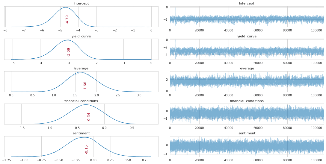
pm.summary(trace_mh)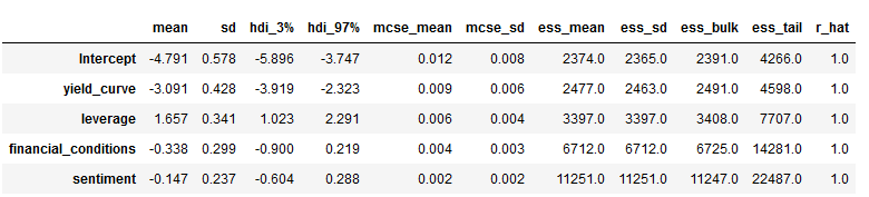
NUTSサンプラー
サンプリング方法を指定せずにpm.sampleを使用すると、デフォルトでNo U-Turn Samplerに設定されます。これは、パラメーターを自動的に調整するハミルトニアンモンテカルロの形式です。通常は、バニラメトロポリスヘイスティングスと比較して、収束が速く、相関性の低いサンプルが得られます。
非常に異なるスケールで測定された変数は、サンプリングプロセスを遅くする可能性があることに注意してください。したがって、最初にsklearnのscale()関数を適用して、変数age,hours,educを標準化します。
少数のサンプルを描く
新しい式で上記のようにモデルを定義したら、事後分布を近似するための推論を実行する準備が整います。 MCMCサンプリングアルゴリズムは、pm.sample()関数を介して使用できます。
デフォルトでは、PyMC3は最も効率的なサンプラーを自動的に選択し、効率的な収束のためにサンプリングプロセスを初期化します。連続モデルの場合、PyMC3は前のセクションで説明したNUTSサンプラーを選択します。また、ADVIを介して変分推論を実行し、サンプラーの適切な開始パラメーターを見つけます。いくつかの選択肢の1つは、MAP推定値を使用することです。
収束がどのように見えるかを確認するために、サンプラーを1,000回反復して破棄した後、最初に100個のサンプルのみを描画します。 cores引数を使用して、サンプリングプロセスを複数のチェーンに対して並列化できます(GPUを使用する場合を除く)。
draws = 100
tune = 1000
with logistic_model:
   trace_NUTS = pm.sample(draws=draws,
                          tune=tune,
                          init='adapt_diag',
                          chains=4,
                          cores=1,
                          random_seed=42)
'''
Only 100 samples in chain.
Auto-assigning NUTS sampler...
Initializing NUTS using adapt_diag...
Sequential sampling (4 chains in 1 job)
NUTS: [sentiment, financial_conditions, leverage, yield_curve, Intercept]
'''
trace_df = pm.trace_to_dataframe(trace_NUTS).assign(
chain=lambda x: x.index // draws)
trace_df.info()
'''
<class 'pandas.core.frame.DataFrame'>
RangeIndex: 400 entries, 0 to 399
Data columns (total 6 columns):
# Column Non-Null Count Dtype
--- ------ -------------- -----
0 Intercept 400 non-null float64
1 yield_curve 400 non-null float64
2 leverage 400 non-null float64
3 financial_conditions 400 non-null float64
4 sentiment 400 non-null float64
5 chain 400 non-null int64
dtypes: float64(5), int64(1)
memory usage: 18.9 KB
'''plot_traces(trace_NUTS, burnin=0)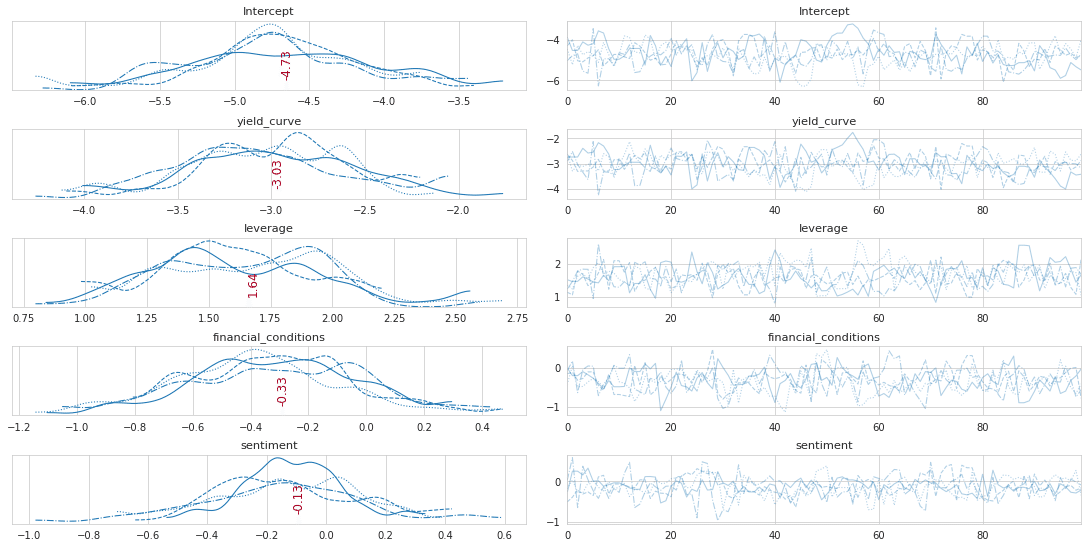
draws = 50000
chains = 4
with logistic_model:
   trace_NUTS = pm.sample(draws=draws,
                          tune=tune,
                          init='adapt_diag',
                          trace=trace_NUTS,
                          chains=chains,
                          cores=1,
                          random_seed=42)
'''
Auto-assigning NUTS sampler...
Initializing NUTS using adapt_diag...
Sequential sampling (4 chains in 1 job)
NUTS: [sentiment, financial_conditions, leverage, yield_curve, Intercept]
'''
plot_traces(trace_NUTS, burnin=1000)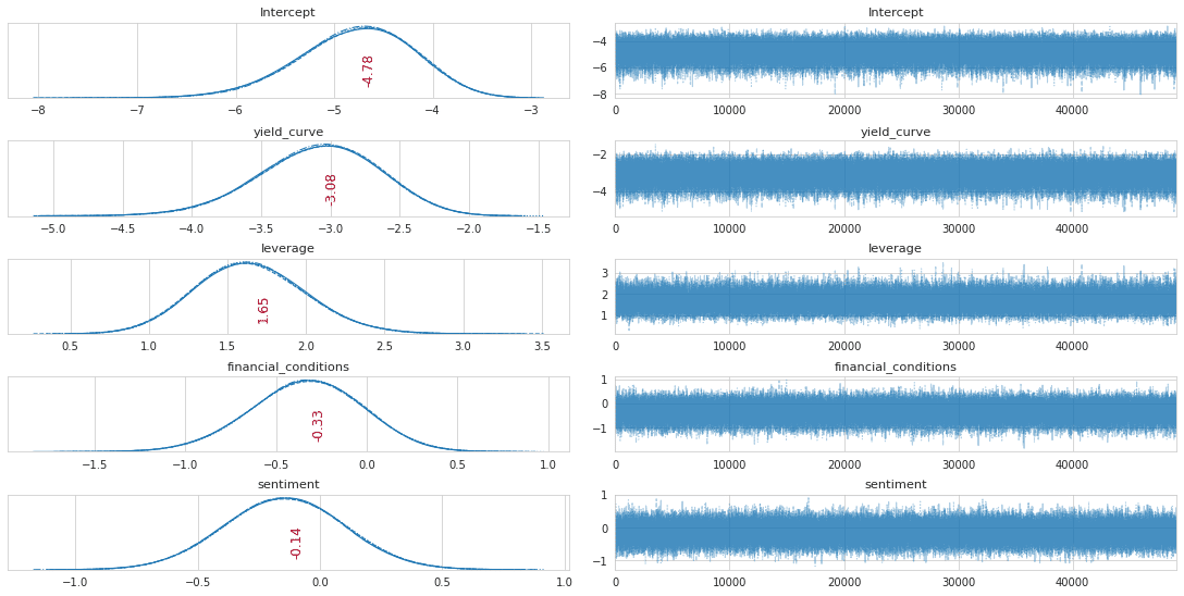
経過を組み合わせる
df = pm.trace_to_dataframe(trace_NUTS).iloc[200:].reset_index(
   drop=True).assign(chain=lambda x: x.index // draws)
trace_df = pd.concat([trace_df.assign(samples=100),
                     df.assign(samples=len(df) + len(trace_df))])
trace_df.info()
'''
<class 'pandas.core.frame.DataFrame'>
Int64Index: 200600 entries, 0 to 200199
Data columns (total 7 columns):
#   Column                Non-Null Count   Dtype
---  ------                --------------   -----
0   Intercept             200600 non-null  float64
1   yield_curve           200600 non-null  float64
2   leverage              200600 non-null  float64
3   financial_conditions  200600 non-null  float64
4   sentiment             200600 non-null  float64
5   chain                 200600 non-null  int64
6   samples               200600 non-null  int64
dtypes: float64(5), int64(2)
memory usage: 12.2 MB
'''
両方の経過を視覚化する
trace_df_long = pd.melt(trace_df, id_vars=['samples', 'chain'])
trace_df_long.info()
'''
<class 'pandas.core.frame.DataFrame'>
RangeIndex: 1003000 entries, 0 to 1002999
Data columns (total 4 columns):
#   Column    Non-Null Count    Dtype
---  ------    --------------    -----
0   samples   1003000 non-null  int64
1   chain     1003000 non-null  int64
2   variable  1003000 non-null  object
3   value     1003000 non-null  float64
dtypes: float64(1), int64(2), object(1)
memory usage: 30.6+ MB
'''
g = sns.FacetGrid(trace_df_long, col='variable', row='samples',
hue='chain', sharex='col', sharey=False)
g = g.map(sns.distplot, 'value', hist=False, rug=False);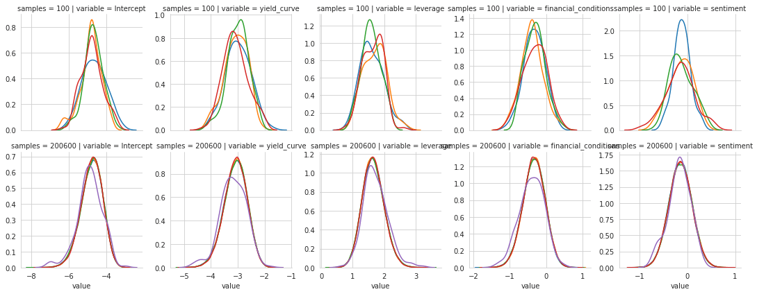
model = smf.logit(formula=full_model, data=data)
result = model.fit()
print(result.summary())
'''
Optimization terminated successfully.
        Current function value: 0.185828
        Iterations 9
                          Logit Regression Results
==============================================================================
Dep. Variable:              recession   No. Observations:                  445
Model:                          Logit   Df Residuals:                      440
Method:                           MLE   Df Model:                            4
Date:                Thu, 13 Aug 2020   Pseudo R-squ.:                  0.4847
Time:                        07:09:54   Log-Likelihood:                -82.693
converged:                       True   LL-Null:                       -160.47
Covariance Type:            nonrobust   LLR p-value:                 1.312e-32
========================================================================================
                          coef    std err          z      P>|z|      [0.025      0.975]
----------------------------------------------------------------------------------------
Intercept               -4.5897      0.554     -8.279      0.000      -5.676      -3.503
yield_curve             -2.9559      0.412     -7.169      0.000      -3.764      -2.148
leverage                 1.5767      0.331      4.758      0.000       0.927       2.226
financial_conditions    -0.3010      0.294     -1.024      0.306      -0.877       0.275
sentiment               -0.1389      0.233     -0.596      0.551      -0.596       0.318
========================================================================================
'''pm.summary(trace_NUTS).assign(statsmodels=result.params).to_csv(model_path / 'trace_nuts.csv')pm.summary(trace_NUTS).assign(statsmodels=result.params)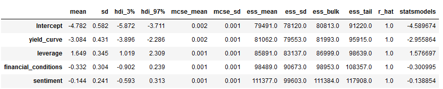
信頼区間を計算する。
トレースのパーセンタイルとして、信頼できる区間(ベイズ推定における信頼区間)を計算できます。結果の境界は、パラメーターが多数の試行でこの範囲内にある回数とは対照的に、特定の確率の敷居値のパラメーター値の範囲についての確信を反映しています。
def get_credible_int(trace, param):
   b = trace[param]
   lb, ub = np.percentile(b, 2.5), np.percentile(b, 97.5)
   lb, ub = np.exp(lb), np.exp(ub)
   return b, lb, ub
b = trace_NUTS['yield_curve']
lb, ub = np.percentile(b, 2.5), np.percentile(b, 97.5)
lb, ub = np.exp(lb), np.exp(ub)
print(f'P({lb:.3f} < Odds Ratio < {ub:.3f}) = 0.95')
'''
P(0.019 < Odds Ratio < 0.101) = 0.95
'''b, lb, ub = get_credible_int(trace_NUTS, 'yield_curve')
print(f'P({lb:.3f} < Odds Ratio < {ub:.3f}) = 0.95')
'''
P(0.019 < Odds Ratio < 0.101) = 0.95
'''fig, axes = plt.subplots(figsize=(14, 4), ncols=2)
b, lb, ub = get_credible_int(trace_NUTS, 'yield_curve')
sns.distplot(np.exp(b), axlabel='Odds Ratio', ax=axes[0])
axes[0].set_title(f'Yield Curve: P({lb:.3f} < Odds Ratio < {ub:.3f}) = 0.95')
axes[0].axvspan(lb, ub, alpha=0.5, color='gray')
b, lb, ub = get_credible_int(trace_NUTS, 'leverage')
sns.distplot(np.exp(b), axlabel='Odds Ratio', ax=axes[1])
axes[1].set_title(f'Leverage: P({lb:.3f} < Odds Ratio < {ub:.3f}) = 0.95')
axes[1].axvspan(lb, ub, alpha=0.5, color='gray')
fig.suptitle('Credible Intervals', fontsize=14)
sns.despine()
fig.tight_layout()
fig.subplots_adjust(top=.9);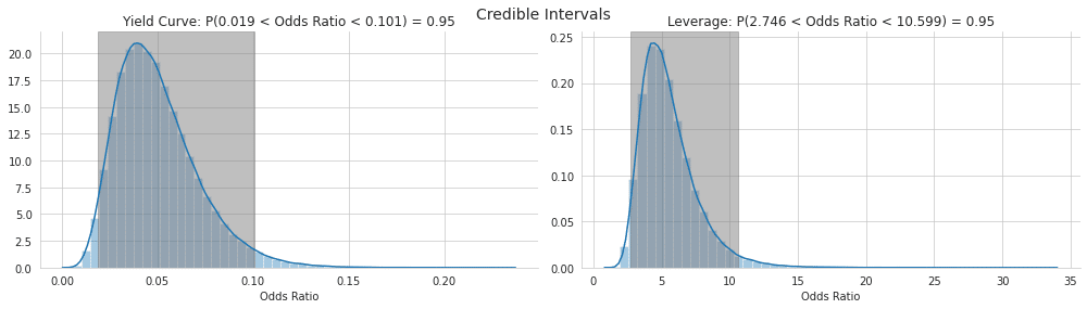
変分推論
ADVI(Automatic Differentiation Variational Inference)を実行する
変分推論のインターフェイスは、MCMCの実装と非常に似ています。 sample()関数の代わりにfit()を使用するだけで、分布適合プロセスが特定の許容範囲に収束した場合に、早期停止CheckParametersConvergenceコールバックを含めるオプションがあります。
with logistic_model:
   callback = CheckParametersConvergence(diff='absolute')
   approx = pm.fit(n=100000,
                   callbacks=[callback])
近似分布からのサンプル
上記のMCMCサンプラーのように、近似分布からサンプルを描画してトレースオブジェクトを取得できます。
trace_advi = approx.sample(10000)pm.summary(trace_advi)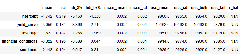
pm.summary(trace_advi).to_csv(model_path / 'trace_advi.csv')モデルの診断
ベイジアンモデル診断には、サンプリングプロセスが収束し、一貫して事後の高確率領域からサンプリングされていることの検証、およびモデルがデータを適切に表していることの確認が含まれます。
多くの変数を持つ高次元モデルの場合、トレースで多数を検査するのは面倒になります。 NUTSを使用する場合、エネルギープロットは収束の問題を評価するのに役立ちます。これは、ランダムプロセスが効率的に事後を探索する方法を要約しています。プロットは、次の例のようによく一致するはずのエネルギーとエネルギー遷移行列を示しています(概念の詳細については、参照を参照してください)。
エネルギープロット
pm.energyplot(trace_NUTS);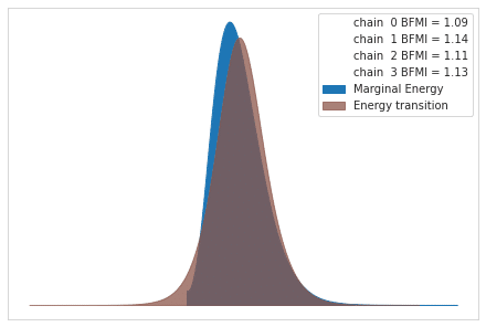
フォレストプロット
pm.forestplot(trace_NUTS);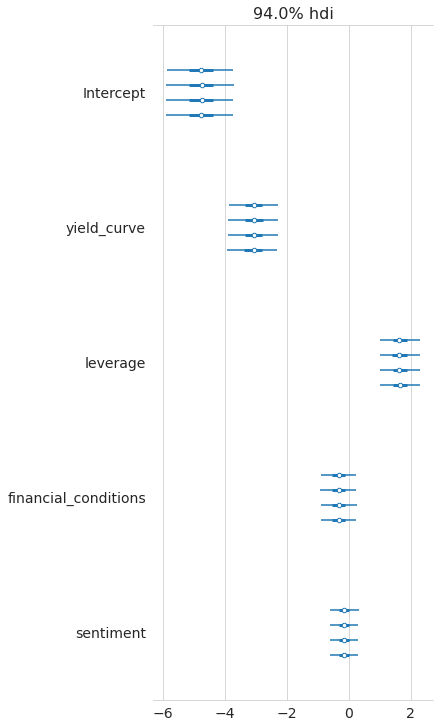
fig, axes = plt.subplots(ncols=2, figsize=(14, 4))
pm.forestplot(trace_NUTS, ax=axes[0])
axes[0].set_title('Forest Plot')

pm.energyplot(trace_NUTS, ax=axes[1])
axes[1].set_title('Energy Plot')

fig.tight_layout();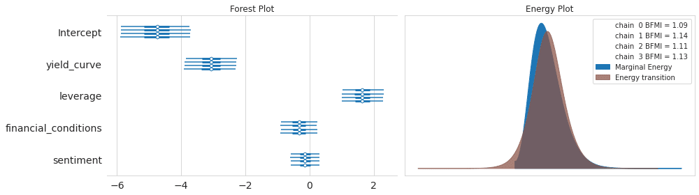
事後予測確認
PPCは、モデルがデータにどれだけ適合するかを調べるのに非常に役立ちます。それらは、事後からのドローからのパラメーターを使用してモデルからデータを生成することによって行います。この目的のために関数pm.sample_ppcを使用し、観測ごとにn個のサンプルを取得します(GLMモジュールは結果に自動的にyという名前を付けます):
ppc = pm.sample_posterior_predictive(trace_NUTS, samples=500, model=logistic_model)ppc['y'].shape
'''
(500, 445)
'''y_score = np.mean(ppc['y'], axis=0)roc_auc_score(y_score=np.mean(ppc['y'], axis=0),
y_true=data.recession)
'''
0.9428948913681738
'''予測
予測では、theanoの共有変数を使用して、事後予測チェックを実行する前に訓練データをテストデータに置き換えます。視覚化を容易にするために、単一の予測時間で変数を作成し、トレーニングおよびテストデータセットを作成し、前者を共有変数に変換します。 numpy配列を使用し、列ラベルのリストを提供する必要があることに注意してください。
訓練ーテスト 分離
X = data[['yield_curve']]
labels = X.columns
y = data.recession
X_train, X_test, y_train, y_test = train_test_split(X, y,
                                                   test_size=0.2,
                                                   random_state=42,
                                                   stratify=y)
theanoの共有変数を作成
X_shared = theano.shared(X_train.values)ロジスティックモデルの定義
with pm.Model() as logistic_model_pred:
   pm.glm.GLM(x=X_shared,
              labels=labels,
              y=y_train,
              family=pm.glm.families.Binomial())
NUTSサンプラーの実行
with logistic_model_pred:
   pred_trace = pm.sample(draws=10000,
                          tune=1000,
                          chains=2,
                          cores=1,
                          init='adapt_diag')
'''
Auto-assigning NUTS sampler...
Initializing NUTS using adapt_diag...
Sequential sampling (2 chains in 1 job)
NUTS: [yield_curve, Intercept]
'''
共有変数をテストセットに置き換える
前と同じようにサンプラーを実行し、訓練をテストデータで置き換えた後、結果のトレースにpm.sample_ppc関数を適用します。
X_shared.set_value(X_test)ppc = pm.sample_posterior_predictive(pred_trace,
model=logistic_model_pred,
samples=100)AUCスコアの確認
y_score = np.mean(ppc['y'], axis=0)
roc_auc_score(y_score=np.mean(ppc['y'], axis=0),
             y_true=y_test)
'''
0.840506329113924
'''
def invlogit(x):
return np.exp(x) / (1 + np.exp(x))x = X_test.yield_curve
fig, ax = plt.subplots(figsize=(14, 5))
β = stats.beta((ppc['y'] == 1).sum(axis=0), (ppc['y'] == 0).sum(axis=0))
# estimated probability
ax.scatter(x=x, y=β.mean())
# error bars on the estimate
plt.vlines(x, *β.interval(0.95))
# actual outcomes
ax.scatter(x=x, y=y_test, marker='x')
# True probabilities
x_ = np.linspace(x.min()*1.05, x.max()*1.05, num=100)
ax.plot(-x_, invlogit(x_), linestyle='-')
ax.set_xlabel('Yield Curve')
ax.set_ylabel('Recession')
ax.invert_xaxis()
fig.tight_layout();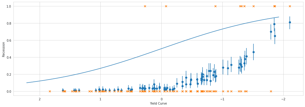
MCMCサンプラーアニメーション
こちらはほぼおまけですので、詳しくは公式ドキュメント(MCMC visualization tutorial)をご参照ください。
この記事が気に入ったらサポートをしてみませんか?