
第10章:ベイジアンML-ダイナミックSR 第4節: ローリング回帰

はじめに
第9章では、共和分に基づくペアトレーディングを紹介しました。
重要な実装ステップは、相殺する位置の相対的なサイズを決定するためのヘッジ比率の推定を含みました。
ここでは、ローリングベイズ線形回帰を使用してこの比率を計算する方法について説明します。
インポートと設定
import warnings
warnings.filterwarnings('ignore')
%matplotlib inline
from pathlib import Path
import numpy as np
import theano
import pymc3 as pm
from sklearn.preprocessing import scale
import yfinance as yf
import matplotlib.pyplot as plt
import seaborn as sns# model_path = Path('models')
sns.set_style('whitegrid')単純線形回帰デモ
人口データ
size = 200
true_intercept = 1
true_slope = 2

x = np.linspace(0, 1, size)
true_regression_line = true_intercept + true_slope * x
y = true_regression_line + np.random.normal(scale=.5, size=size)

x_shared = theano.shared(x)
モデル定義
with pm.Model() as linear_regression: # model specification

   # Define priors
   sd = pm.HalfCauchy('sigma', beta=10, testval=1) # unique name for each variable
   intercept = pm.Normal('intercept', 0, sd=20)
   slope = pm.Normal('slope', 0, sd=20)

   # Define likelihood
likelihood = pm.Normal('y', mu=intercept + slope * x_shared, sd=sd, observed=y)pm.model_to_graphviz(linear_regression)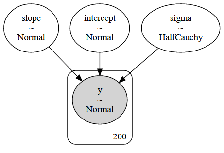
HMC推定
with linear_regression:
   # Inference
   trace = pm.sample(draws=2500, # draw 2500 samples from posterior using NUTS sampling
                     tune=1000,
cores=1) pm.plot_posterior(trace);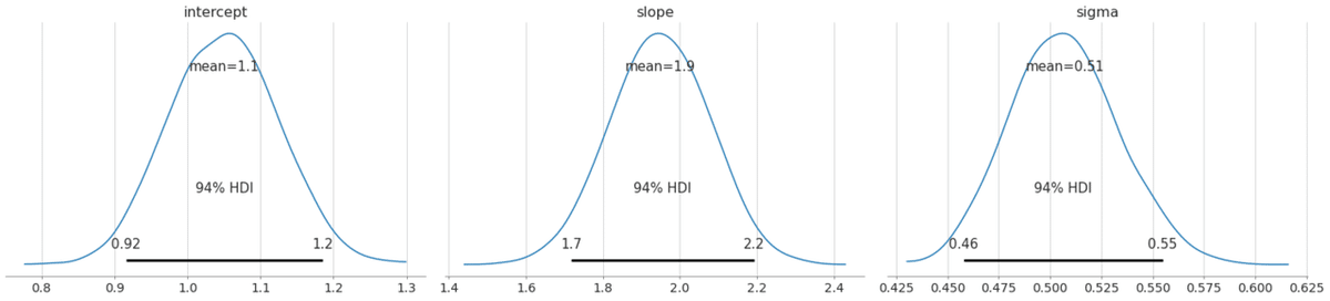
ペアトレーディングで線形回帰
prices = yf.download('GFI GLD', period='max').dropna().loc[:, 'Close']
'''
[*********************100%***********************]  2 of 2 completed
'''
returns = prices.pct_change().dropna()prices.info()
'''
<class 'pandas.core.frame.DataFrame'>
DatetimeIndex: 3962 entries, 2004-11-18 to 2020-08-14
Data columns (total 2 columns):
# Column Non-Null Count Dtype
--- ------ -------------- -----
0 GFI 3962 non-null float64
1 GLD 3962 non-null float64
dtypes: float64(2)
memory usage: 92.9 KB
'''returns.info()
'''
<class 'pandas.core.frame.DataFrame'>
DatetimeIndex: 3961 entries, 2004-11-19 to 2020-08-14
Data columns (total 2 columns):
# Column Non-Null Count Dtype
--- ------ -------------- -----
0 GFI 3961 non-null float64
1 GLD 3961 non-null float64
dtypes: float64(2)
memory usage: 92.8 KB
'''prices_normed = prices.apply(scale)時間の経過とともに価格をプロットすると、強い相関関係が示唆されます。ただし、相関関係は時間とともに変化するようです。
fig, axes= plt.subplots(figsize=(14,4), ncols=2)

prices.plot(secondary_y='GFI', ax=axes[0])
axes[0].set_title('Asset Price Series')
points = axes[1].scatter(prices.GLD,
                        prices.GFI,
                        c=np.linspace(0.1, 1, len(prices)),
                        s=15,
                        cmap='winter')
axes[1].set_title('Price Correlation over Time')
cbar = plt.colorbar(points, ax=axes[1])
cbar.ax.set_yticklabels([str(p.year) for p in returns[::len(returns)//10].index]);

sns.regplot(x='GLD', y='GFI',
           data=prices,
           scatter=False,
           color='k',
           line_kws={'lw':1,
                     'ls':'--'},
           ax=axes[1])
sns.despine()
fig.tight_layout();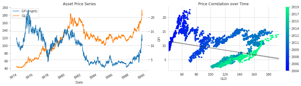
with pm.Model() as model_reg:
   pm.glm.GLM.from_formula('GFI ~ GLD', prices)
   trace_reg = pm.sample(draws=5000,
                         tune=1000,
                         cores=1)
fig = plt.figure(figsize=(10, 5))
ax = fig.add_subplot(111,
xlabel='GLD',
ylabel='GFI',
title='Posterior predictive regression lines')
points = ax.scatter(prices.GLD,
prices.GFI,
c=np.linspace(0.1, 1, len(prices)),
s=15,
cmap='winter')
pm.plot_posterior_predictive_glm(trace_reg[100:],
samples=250,
label='posterior predictive regression lines',
lm=lambda x,
sample: sample['Intercept'] + sample['GLD'] * x,
eval=np.linspace(prices.GLD.min(), prices.GLD.max(), 100))
cb = plt.colorbar(points)
cb.ax.set_yticklabels([str(p.year) for p in prices[::len(prices)//10].index]);
ax.legend(loc=0);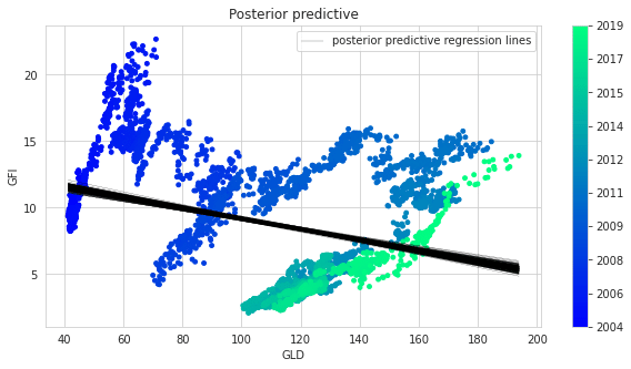
ローリング回帰
次に、時間の経過に伴う回帰係数の変化を可能にする改善されたモデルを構築します。具体的には、切片と傾きが時間のランダムウォークに従うと仮定します。
αt ~ N(α_{t-1}, σ_{α}^2)
βt ~ N(β_{t-1}, σ_{β}^2)
まず、σ_{α}とσ_{β}のハイパー優先度を定義しましょう。
このパラメーターは、回帰係数のボラティリティとして解釈できます。
model_randomwalk = pm.Model()
with model_randomwalk:
   sigma_alpha = pm.Exponential('sigma_alpha', 50.)
   alpha = pm.GaussianRandomWalk('alpha',
                                 sd=sigma_alpha,
                                 shape=len(prices))

   sigma_beta = pm.Exponential('sigma_beta', 50.)
   beta = pm.GaussianRandomWalk('beta',
                                sd=sigma_beta,
                                shape=len(prices))
with model_randomwalk:
# Define regression
regression = alpha + beta * prices_normed.GLD
# Assume prices are normally distributed
# Get mean from regression.
sd = pm.HalfNormal('sd', sd=.1)
likelihood = pm.Normal('y',
mu=regression,
sd=sd,
observed=prices_normed.GFI)with model_randomwalk:
trace_rw = pm.sample(tune=2000,
draws=200,
cores=1,
target_accept=.9)結果の分析
fig, axes = plt.subplots(figsize=(15, 5), ncols=2, sharex=True)

axes[0].plot(trace_rw['alpha'].T, 'r', alpha=.05)
axes[0].set_xlabel('Time')
axes[0].set_ylabel('Alpha')
axes[0].set_title('Intercept')
axes[0].set_xticklabels([str(p.date()) for p in prices[::len(prices)//9].index])

axes[1].plot(trace_rw['beta'].T, 'b', alpha=.05)
axes[1].set_xlabel('Time')
axes[1].set_ylabel('Beta')
axes[1].set_title('Slope')

fig.suptitle('Changes of coefficients over time', fontsize=14)
sns.despine()
fig.tight_layout()
fig.subplots_adjust(top=.9);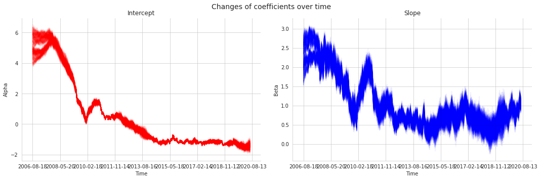
事後予測プロットは、時間の経過に伴う回帰の変化をより適切に捉えていることを示しています。価格の代わりに返品を使用する必要があったことに注意してください。モデルは同じように機能しますが、視覚化はそれほど明確ではありません。
x = np.linspace(prices_normed.GLD.min(),
                prices_normed.GLD.max())

dates = [str(p.year) for p in prices[::len(prices)//9].index]

colors = np.linspace(0.1, 1, len(prices))
colors_sc = np.linspace(0.1, 1, len(trace_rw[::10]['alpha'].T))

cmap = plt.get_cmap('winter')
fig, ax = plt.subplots(figsize=(14, 8))
for i, (alpha, beta) in enumerate(zip(trace_rw[::25]['alpha'].T,
trace_rw[::25]['beta'].T)):
for a, b in zip(alpha[::25], beta[::25]):
ax.plot(x,
a + b*x,
alpha=.01,
lw=.5,
c=cmap(colors_sc[i]))
points = ax.scatter(prices_normed.GLD,
prices_normed.GFI,
c=colors,
s=5,
cmap=cmap)
cbar = plt.colorbar(points)
cbar.ax.set_yticklabels(dates);
ax.set_xlabel('GLD')
ax.set_ylabel('GFI')
ax.set_title('Posterior predictive regression lines')
sns.despine()
fig.tight_layout();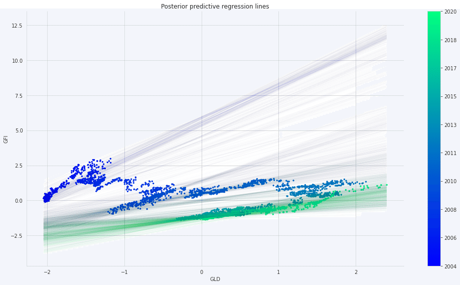
この記事が気に入ったらサポートをしてみませんか?