
第11章:ランダムフォレスト - ロングショート戦略 第2節: バギング決定木(バギングが予測バリアンスをどう削減するのか)

インポートと設定
import warnings
warnings.filterwarnings('ignore')
%matplotlib inline
from pathlib import Path
import numpy as np
from numpy.random import choice, normal
import pandas as pd
import matplotlib.pyplot as plt
import seaborn as sns
from sklearn.tree import DecisionTreeRegressor
from sklearn.ensemble import BaggingRegressorsns.set_style('white')
np.random.seed(seed=42)results_path = Path('results', 'random_forest')
if not results_path.exists():
results_path.mkdir(parents=True)バギングされた決定木
決定木にバギングを適用するには、置換で繰り返しサンプリングして訓練データからブートストラップサンプルを作成し、次にこれらの各サンプルで1つの決定木をトレーニングし、さまざまなツリーの予測を平均してアンサンブル予測を作成します。
バギングされた決定木は通常大きく成長します。つまり、多くの層と葉のノードがあり、枝刈りされないため、各ツリーのバイアスは低くなりますが分散は高くなります。次に、それらの予測を平均化する効果は、それらの分散を減らすことを目的としています。バギングは、ブートストラップサンプルで訓練された数百または数千ものツリーを組み合わせたアンサンブルを構築することにより、予測パフォーマンスを大幅に向上させることが示されています。
回帰ツリーの分散に対するバギングの影響を説明するために、sklearnが提供するBaggingRegressorメタ推定器を使用できます。サンプリング戦略を指定するパラメーターに基づいて、ユーザー定義の基本推定量をトレーニングします。
・max_samplesとmax_featuresは、それぞれ行と列から描画されるサブセットのサイズを制御します。
・bootstrapとbootstrap_featuresは、これらの各サンプルが置き換えの有無で描画されるかどうかを決定します。
学習用曲線
def f(x):
   return np.exp(-(x+2) ** 2) + np.cos((x-2)**2)

x = np.linspace(-3, 2, 1000)
y = pd.Series(f(x), index=x)
y.plot(title='Wiggly Exponential Function')
sns.despine()
plt.tight_layout();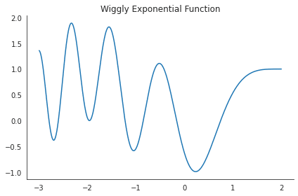
訓練のシミュレーション
次の例では、前述の指数関数f(x)を使用して、1つのDecisionTreeRegressorと、それぞれが10レベルの深さで成長する10本のツリーで構成されるBaggingRegressor集団のトレーニングサンプルを生成します。両方のモデルはランダムサンプルでトレーニングされ、ノイズが追加された実際の関数の結果を予測します。
真の関数がわかっているので、平均二乗誤差をバイアス、分散、ノイズに分解し、次の分類に従って両方のモデルのこれらのコンポーネントの相対的なサイズを比較できます。
100回の反復ランダムトレーニングと250回および500回の観測のテストサンプルの場合、個々の決定木の予測の分散は、ブートストラップされたサンプルに基づく10個のバギングされた木の小さな集団の分散のほぼ2倍であることがわかります。
test_size = 500
train_size = 250
reps = 100

noise = .5  # noise relative to std(y)
noise = y.std() * noise

X_test = choice(x, size=test_size, replace=False)

max_depth = 10
n_estimators=10

tree = DecisionTreeRegressor(max_depth=max_depth)
bagged_tree = BaggingRegressor(base_estimator=tree, n_estimators=n_estimators)
learners = {'Decision Tree': tree, 'Bagging Regressor': bagged_tree}

predictions = {k: pd.DataFrame() for k, v in learners.items()}
for i in range(reps):
   X_train = choice(x, train_size)
   y_train = f(X_train) + normal(scale=noise, size=train_size)
   for label, learner in learners.items():
       learner.fit(X=X_train.reshape(-1, 1), y=y_train)
       preds = pd.DataFrame({i: learner.predict(X_test.reshape(-1, 1))}, index=X_test)
       predictions[label] = pd.concat([predictions[label], preds], axis=1)
# y only observed with noise
y_true = pd.Series(f(X_test), index=X_test)
y_test = pd.DataFrame(y_true.values.reshape(-1,1) + normal(scale=noise, size=(test_size, reps)), index=X_test)result = pd.DataFrame()
for label, preds in predictions.items():
result[(label, 'error')] = preds.sub(y_test, axis=0).pow(2).mean(1) # mean squared error
result[(label, 'bias')] = y_true.sub(preds.mean(axis=1), axis=0).pow(2) # bias
result[(label, 'variance')] = preds.var(axis=1)
result[(label, 'noise', )] = y_test.var(axis=1)
result.columns = pd.MultiIndex.from_tuples(result.columns)df = result.mean().sort_index().loc['Decision Tree']
f"{(df.error- df.drop('error').sum()) / df.error:.2%}"
'''
'0.29%'
'''df = result.mean().sort_index().loc['Bagging Regressor']
f"{(df.error- df.drop('error').sum()) / df.error:.2%}"
'''
'0.25%'
'''バイアスーバリアンス 資格化ブレイクダウン
次のプロットは、各モデルについて、上部パネルに両方のモデルの平均予測と2つの標準偏差の帯(band)、下部パネルにある真の関数の値に基づくバイアス、バリアンス、ノイズの内訳を示しています。
fig, axes = plt.subplots(ncols=2, nrows=2, figsize=(14, 7), sharex=True, sharey='row')
axes = axes.flatten()
idx = pd.IndexSlice

for i, (model, data) in enumerate(predictions.items()):
   mean, std = data.mean(1), data.std(1).mul(2)
   (pd.DataFrame([mean.sub(std), mean, mean.add(std)]).T
    .sort_index()
    .plot(style=['k--', 'k-', 'k--'], ax=axes[i], lw=1, legend=False, ylim=(-2, 3)))
   (data.stack().reset_index()
    .rename(columns={'level_0': 'x', 0: 'y'})
    .plot.scatter(x='x', y='y', ax=axes[i], alpha=.02, s=2, color='r', title=model))
   r = result[model]
   m = r.mean()
   kwargs = {'transform': axes[i].transAxes, 'fontsize':10}
   axes[i].text(x=.8, y=.9, s=f'Bias: {m.bias:.2%}', **kwargs)
   axes[i].text(x=.75, y=.8, s=f'Variance: {m.variance:.2%}', **kwargs)

   (r.drop('error', axis=1).sort_index()
    .rename(columns=str.capitalize)
    .plot(ax=axes[i+2], lw=1, legend=False, stacked=True, ylim=(0, .4)))

axes[-1].legend(fontsize=10)
fig.suptitle('Bias-Variance Breakdown', fontsize=14)
sns.despine()
fig.tight_layout()
fig.subplots_adjust(top=.93);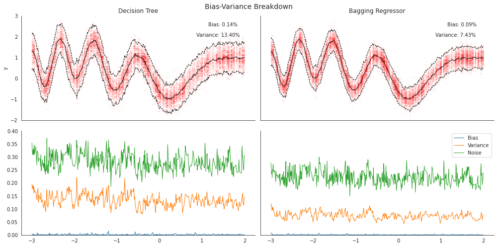
この記事が気に入ったらサポートをしてみませんか?