Pythonで多角形のアリアを計算する。numpy、Shapley, OpenCV

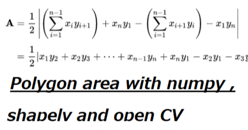
Shoelace Formula 座標法（ざひょうほう）

多角形のアリアを計算するために、一般的に Shoelaceの方程式　（日本語で 座標法）を使用します。

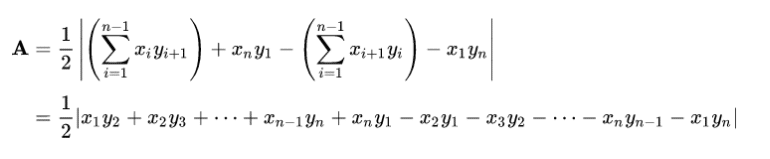
複雑そうな方程式ですが、本当に靴ひものような計算し方です。Xは靴ひもの左側とYが右側で交差的に合計を算出されています。

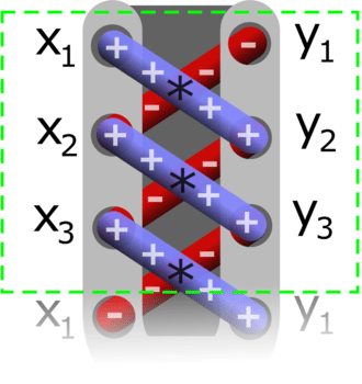
 Pythonでこのような機能は、np.roll(a,shift, axis=None)という関数ができます。下記は、numpyを使用し、 Shoelaceの方程式です。例の多角形は、XとYの部分に分ければ、アリアを計算できます。

import numpy as np
def PolyArea(x,y):
   return 0.5*np.abs(np.dot(x,np.roll(y,1))-np.dot(y,np.roll(x,1)))
   
 #レイの多角形 points=[[  0, 200],
       [200,   0],
       [200, 100],
       [100, 100],
       [100, 200]]
x,y=points[:,0],points[:,1]
print(PolyArea(x,y)
) #10000.0 

Shapelyというモジュールでは、多角形の扱いはもっと適用です。上記の関数を使用なしで、簡単にアリアを計算できます。

from shapely.geometry import Polygon
Poly = Polygon(zip(x, y)) 
print(Poly.area)  #10000.0 

バルーンのアリアを抽出 (Open CV)

画像解析では、画像から物体を抽出し、特徴を計算する問題が一般的です。例えば、物体Xのアリアなど。上記のコードを使用すれば、抽出された物体のアリアを計算できますね。しかし、その物体を抽出し、多角形を包まなければなりません。そのために、Open CVを使用します。

上記のバルーンの写真を使用しましょう。抽出するために、色画像からHSVの画像を変換すれば、もっと簡単になります。下記のコードでは、その通りにして、ヒストグラムでHSVの値を分解します。

file="balloon.jpg"
img=cv2.imread(file)[:,:,::-1] #RGB -> BGR 
 
hsvim = cv2.cvtColor(img, cv2.COLOR_BGR2HSV)
fig,axs=plt.subplots(1,3,figsize=(10,10))

for b in range(3):
 axs[b].imshow(hsvim[:,:,b])
 axs[b].set_title(f"band-{b}")

def hist_color_img(img,bands,ax=None,range=None): 
 if not ax: 
   fig,ax=plt.subplots(1,1,figsize=(8,6)) 
 print(bands) 
 for band in bands: 
    print(f"band-{band}") 
    _= ax.hist(img[:,:,band].reshape(-1),bins=20,label=f"band-{band}",alpha=0.8,range=range) 
 ax.legend() 
 ax.grid() 
 #plt.show() 
hist_color_img(hsvim,[0,1,2])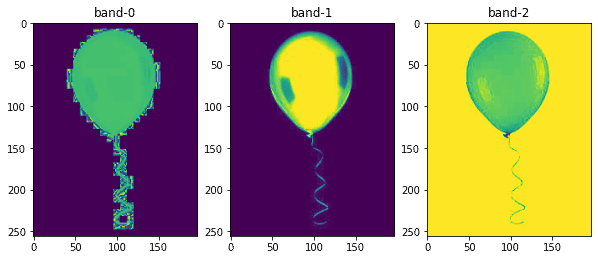

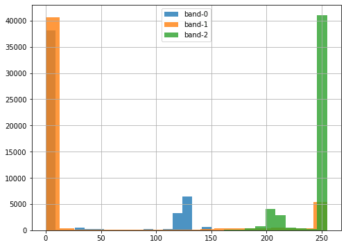
その結果から、band-2（V）では、使用しやすいしきい値がはっきり見えます。次に、cv2.thresholdを使用し、この閾値からバルーンの二値化をします。その二値化画像は、 cv2.findContours(thresh, 1, 3)を行ると輪郭を抽出し、一番大きいな輪郭はバルーンの物体でしょう。その物体を認識して、Shapleyで多角形に変換して、バルーンのアリアを簡単に計算できます。

 #バルーンの範囲を抽出する lower = np.array([0, 0, 0], dtype = "uint8")
upper = np.array([255, 255, 240], dtype = "uint8")
RegionHSV = cv2.inRange(hsvim, lower, upper)
ret,thresh = cv2.threshold(~RegionHSV,0,255,cv2.THRESH_BINARY)

 #輪郭をゲット contours, hierarchy = cv2.findContours(thresh, 1, 3)
contours=list([c for c in contours if len(c)>2]) #Only Polygons not points 
print(len(contours))
#ballon area only -> back out background 
out_img=cv2.bitwise_or(img, img,mask=~thresh)


 #画像で輪郭を加える 
i=0

for c in contours:
 if len(c)>20:
   print(i,len(c))
   c=c.reshape(1,-1,2)
   

   cv2.polylines(out_img, c, isClosed=True, color=(0, 0, 255), thickness=4)
 i+=1
 
plt.imshow(out_img)

#アリアの計算
balloon_poly=contours[11].reshape( -1, 2)
x,y=balloon_poly[:,0],balloon_poly[:,1]
balloon_poly= Polygon(zip(x, y)) 
print("balloon pixel area",balloon_poly.area)  #b9360.5
plt.title(f"ballon pixel area {balloon_poly.area}")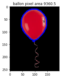

いいですね。バルーンのアリアを計算できました。この簡単な例ですが、機械学習のセグメンテーションのモードを予想された画像では、同じのことを行うと、もっと詳しくデータサイエンスをできますしょう。

そして、皆さんは、この記事の英語版が興味があれば、下記の記事をご覧ください。

Python: Polygon area with numpy , shapely and open CV

すべてのコード

この記事のコードは、GoogleColabのノートブックがあって、コピーしたいなら、すべては下記の通りです。

import shapely 
import numpy as np
import cv2
import matplotlib.pyplot as plt
from shapely.geometry import Polygon


#ランダムの多角形
Random_polygon=np.random.randint(3, size =(2,5))
points=Random_polygon.reshape( 1, -1, 2)*100
img = np.zeros((300, 300, 3), dtype=np.uint8)
cv2.polylines(img, points, isClosed=True, color=(0, 255, 0), thickness=2)
plt.imshow(img)

 #Shoelaceの方程式 def PolyArea(x,y):
   return 0.5*np.abs(np.dot(x,np.roll(y,1))-np.dot(y,np.roll(x,1)))
x,y=points[0][:,0],points[0][:,1]
print(PolyArea(x,y))
randomPoly = Polygon(zip(x, y)) 
print(randomPoly.area) 


 #バルーンの画像を解析 file="balloon.jpg"
img=cv2.imread(file)[:,:,::-1] #RGB -> BGR 
 
hsvim = cv2.cvtColor(img, cv2.COLOR_BGR2HSV)
fig,axs=plt.subplots(1,3,figsize=(10,10))

for b in range(3):
 axs[b].imshow(hsvim[:,:,b])
 axs[b].set_title(f"band-{b}")

def hist_color_img(img,bands,ax=None,range=None): 
 if not ax: 
   fig,ax=plt.subplots(1,1,figsize=(8,6)) 
 print(bands) 
 for band in bands: 
    print(f"band-{band}") 
    _= ax.hist(img[:,:,band].reshape(-1),bins=20,label=f"band-{band}",alpha=0.8,range=range) 
 ax.legend() 
 ax.grid() 
 #plt.show() 
hist_color_img(hsvim,[0,1,2])

 #バルーンの範囲を抽出する lower = np.array([0, 0, 0], dtype = "uint8")
upper = np.array([255, 255, 240], dtype = "uint8")
RegionHSV = cv2.inRange(hsvim, lower, upper)
ret,thresh = cv2.threshold(~RegionHSV,0,255,cv2.THRESH_BINARY)

 #輪郭をゲット contours, hierarchy = cv2.findContours(thresh, 1, 3)
contours=list([c for c in contours if len(c)>2]) #Only Polygons not points 
print(len(contours))
#ballon area only -> back out background 
out_img=cv2.bitwise_or(img, img,mask=~thresh)


 #画像で輪郭を加える 
i=0

for c in contours:
 if len(c)>20:
   print(i,len(c))
   c=c.reshape(1,-1,2)
   

   cv2.polylines(out_img, c, isClosed=True, color=(0, 0, 255), thickness=4)
 i+=1
 
plt.imshow(out_img)

#アリアの計算
balloon_poly=contours[11].reshape( -1, 2)
x,y=balloon_poly[:,0],balloon_poly[:,1]
balloon_poly= Polygon(zip(x, y)) 
print("balloon pixel area",balloon_poly.area)  #b9360.5
plt.title(f"ballon pixel area {balloon_poly.area}")