
Mapleで制御工学の基礎虎の巻6「むだ時間のあるシステムのフィードバック制御」

本記事では、むだ時間のあるシステムにフィードバック制御をしたときのシステムの挙動をナイキスト線図を使って見てみて、ナイキスト線図の結果とステップ応答との関係を見てみたいと思います。
本記事を見るにあたって、Mapleでのナイキスト線図の記事、ステップ応答の記事を事前に読むか理解していることを前提に話を進めます。
本記事で検討するシステムを図1に示します。
一次遅れのプラントモデルの出力をフィードバックして目標値との差分にゲインKをかけてプラントに入力します。ただし、ゲインの出力とプラントへの入力の間にむだ時間L[s]が入っているシステムです。
ゲインK、むだ時間L、一次遅れの時定数τによってシステムの応答は変化します。次にシステムの応答を見てみましょう。
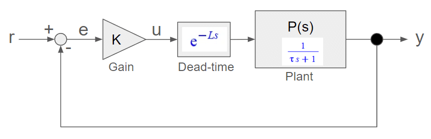
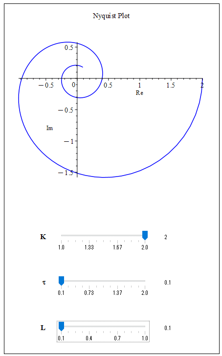
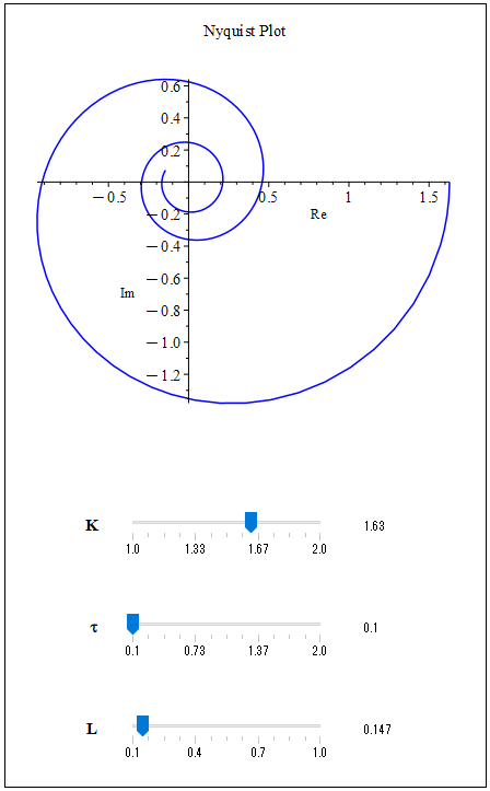
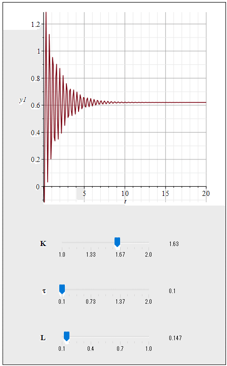
図2はゲインK=2、時定数τ=0.1、むだ時間L=0.1としたときのナイキスト線図です。ナイキスト線図が実軸の「-1」より右を通っているので安定となります。ステップ応答を図3に示していますが、振動はしているものの収束しているのがわかります。でもこんなにシンプルなシステムなのにちょっとむだ時間があるだけで結構な振動をしてしまいます。実際の設計の現場でもむだ時間への対応はしっかり考えておかないと、市場に出てから不具合でも出したら大変なことになります。しっかり検討しておきましょう!

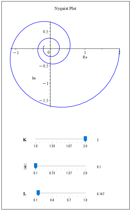
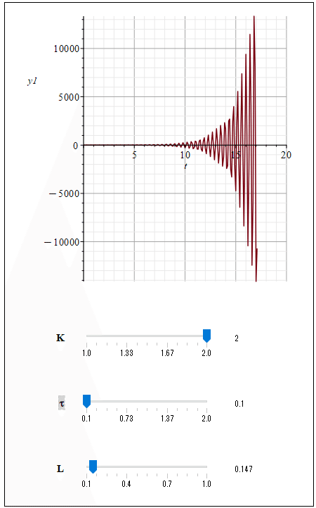
次にむだ時間Lを少しずつ大きくしていくとナイキスト線図が実軸の「-1」より左になってしまいます(図4)。こうするとナイキストの安定判別では不安定となります。この時のステップ応答を図5に示しますが、発散してしまっているのがわかります。むだ時間がわずが0.05[s]弱増えただけで発散してしまいましたね。
そこで今度は、ナイキスト線図が実軸の「-1」より右になるまでゲインを下げていきます(図6)。そうすると図7のステップ応答のように収束するようになります。閉ループ系はむだ時間が大きくなってくると不安定になりますが、ゲインを下げることで安定化させることができます。
まぁ、ゲインを下げることは簡単なことなので知ってか知らずかによらずよくやられる対応ですが、他にもいくつも方法はあるので目的の応答特性になるように、いろいろとチャレンジしてみるとよいでしょう。
ちなみにゲインをもっと下げていくとステップ応答の振動も少なくなっていきます。
さて、先ほどはゲインを下げましたがシステムの時定数を大きくすることによっても、ナイキスト線図が実軸の「-1」より右にさせることもできます(図8)。ステップ応答も収束していますね(図9)。この対策も結構見ますね。制御でうまく安定化できないので、プラント側の動きをゆっくりにさせちゃうという荒業ですね。あまりよい方法ではないので、これはできるだけ避けましょう。


Mapleでむだ時間を含むシステムのナイキスト線図の描き方
以前のナイキスト線図の記事ではコマンド一発でナイキスト線図を描いていましたが、むだ時間がある場合には以下のようなナイキスト線図を手描きするときと同じ手順でプログラムを書く必要があります。プログラム上にコメントも付けているので興味のある方は中身を見てみてください。
restart;
with(plots);

#ラプラス変換の定義 Definition of Laplacevariables
s := 's';

#一次遅れ+むだ時間の伝達関数の定義 Definition of transfer function od first order lag & dead time
G := (K, tau, L) -> K*exp(-L*s)/(tau*s + 1);

#周波数範囲の定義 Frequency Range Definition
omega := 10^(-3) .. 10^2;

#周波数変数の定義 Frequency variables definition
w := 'w';

ReG := (K, tau, L) -> Re(eval(G(K, tau, L), s = w*I));
ImG := (K, tau, L) -> Im(eval(G(K, tau, L), s = w*I));

nyquist_plot := proc(K, tau, L) return plots:-complexplot(ReG(K, tau, L) + ImG(K, tau, L)*I, w = omega, scaling = constrained, title = "Nyquist Plot", labels = ["Re", "Im"], color = blue); end proc;
   return plots:-complexplot(ReG(K, tau, L) + ImG(K, tau, L)*I, w = omega, scaling = constrained, title = "Nyquist Plot", labels = ["Re", "Im"], color = blue)
end proc:

Explore(nyquist_plot(K, tau, L), parameters = [K = 1.0 .. 2.0, tau = 0.1 .. 2, L = 0.1 .. 1.0]);
Mapleでむだ時間を含むシステムのステップ応答の描き方
ステップ応答はナイキスト線図よりもさらに一工夫が必要です。
むだ時間部分をパデ近似して、有理伝達関数にして、プラントモデルと連結し、さらにフィードバック結合をして全体のシステムとします。
それをあとはステップ応答のコマンドで表示させてあげる手順です。
パデ近似の仕方は「むだ時間の伝達関数をパデ近似」の記事を、システムの結合の仕方は「SystemConnectの使い方」の記事を参照してください。
with(DynamicSystems);
with(numapprox);

sysL := L -> TransferFunction(pade(exp(-L*s), s, [3, 3]));
sysP := (K, tau) -> TransferFunction(K/(tau*s + 1));

#直列結合 Series Connect
sysTmp := (K, tau, L) -> SystemConnect(sysP(K, tau), sysL(L), connection = serial);

#フィードバック結合 Feedback Connect
sysAll := (K, tau, L) -> SystemConnect(sysTmp(K, tau, L), 1, connection = negativefeedback);

Explore(ResponsePlot(sysAll(K, tau, L), Step(), duration = 20, gridlines), parameters = [K = 1.0 .. 2.0, tau = 0.1 .. 2, L = 0.1 .. 1.0]);
【English】
In this article, we will look at the behavior of a system when feedback control is applied to a system with dead time, using Nyquist diagrams, and see the relationship between the Nyquist diagram results and step response. In looking at this article, I will assume that you have read or understand the Nyquist diagram article and the step response article in Maple beforehand.
The system considered in this article is shown in Figure 1. The output of the plant model with a first-order delay is fed back and the difference from the target value is multiplied by a gain K and input to the plant. However, the system includes a dead time L[s] between the output of the gain and the input to the plant. The response of the system varies with the gain K, the dead time L, and the time constant τ of the first-order delay. Let us now look at the system response.
Figure 2 shows the Nyquist diagram with gain K = 2, time constant τ = 0.1, and dead time L = 0.1. The Nyquist diagram is stable because it runs to the right of “-1” on the real axis. The step response is shown in Figure 3, and although it oscillates, it is convergent. However, even with such a simple system, just a little dead time can cause a lot of vibration. If you don't think carefully about how to deal with dead time at the actual design, you will be in big trouble if a problem occurs after the product goes on the market. Make sure to consider this carefully!
Next, as the dead time L is gradually increased, the Nyquist diagram becomes left of “-1” on the real axis ( Figure 4 ). In this case, the Nyquist stability discriminant becomes unstable. The step response at this time is shown in Figure 5, and you can see that it has diverged. The system response has diverged even though the dead time has only increased by less than 0.05[s].
So now, the gain is reduced until the Nyquist diagram is to the right of “-1” on the real axis (Figure 6). Then the system will converge as shown in the step response in Figure 7. A closed-loop system becomes unstable as the dead time increases, but it can be stabilized by lowering the gain. Well, lowering the gain is a simple and often done measure, whether you know it or not, but there are many other ways to achieve the desired response characteristics, so it is a good idea to try various methods. Incidentally, as the gain is lowered further, the oscillation in the step response will also decrease.
Now, although the gain was lowered earlier, the Nyquist diagram can also be made to be to the right of “-1” on the real axis by increasing the time constant of the system ( Figure 8). The step response is also converging ( Figure 9). I see this measure quite often. It is a rough trick to slow down the movement of the plant side because the control cannot stabilize it well. This is not a good approach, and should be avoided as much as possible.
How to draw a Nyquist diagram of a system including dead time in Maple
In the previous article on Nyquist diagrams, the Nyquist diagram was drawn with a single command, but for systems with dead time, it is necessary to write a program that follows the same procedure as when drawing Nyquist diagrams by hand, as shown below. I have also added comments on the program, so if you are interested, please take a look at the contents.
restart;
with(plots);

# Definition of Laplacevariables
s := 's';

# Definition of transfer function od first order lag & dead time
G := (K, tau, L) -> K*exp(-L*s)/(tau*s + 1);

# Frequency Range Definition
omega := 10^(-3) .. 10^2;

# Frequency variables definition
w := 'w';

ReG := (K, tau, L) -> Re(eval(G(K, tau, L), s = w*I));
ImG := (K, tau, L) -> Im(eval(G(K, tau, L), s = w*I));

nyquist_plot := proc(K, tau, L) return plots:-complexplot(ReG(K, tau, L) + ImG(K, tau, L)*I, w = omega, scaling = constrained, title = "Nyquist Plot", labels = ["Re", "Im"], color = blue); end proc;
   return plots:-complexplot(ReG(K, tau, L) + ImG(K, tau, L)*I, w = omega, scaling = constrained, title = "Nyquist Plot", labels = ["Re", "Im"], color = blue)
end proc:

Explore(nyquist_plot(K, tau, L), parameters = [K = 1.0 .. 2.0, tau = 0.1 .. 2, L = 0.1 .. 1.0]);
How to draw the step response of a system including dead time in Maple
The step response requires a further twist than the Nyquist diagram. The であd time part is approximated by Pade's approximation, made into a rational transfer function, coupled to the plant model, and then coupled to the feedback coupling to form a whole system. The step response can then be displayed by using the step response command.
Please refer to the article “Padé Approximation of the Transfer Function of the Dead Time” for how to padé approximate and the article “How to Use SystemConnect” for how to connect the system.
with(DynamicSystems);
with(numapprox);

sysL := L -> TransferFunction(pade(exp(-L*s), s, [3, 3]));
sysP := (K, tau) -> TransferFunction(K/(tau*s + 1));

# Series Connect
sysTmp := (K, tau, L) -> SystemConnect(sysP(K, tau), sysL(L), connection = serial);

# Feedback Connect
sysAll := (K, tau, L) -> SystemConnect(sysTmp(K, tau, L), 1, connection = negativefeedback);

Explore(ResponsePlot(sysAll(K, tau, L), Step(), duration = 20, gridlines), parameters = [K = 1.0 .. 2.0, tau = 0.1 .. 2, L = 0.1 .. 1.0]);
【Sample】
Created by Maple 2023.2
この記事が気に入ったらサポートをしてみませんか?