
Mapleで制御工学の基礎虎の巻4「周波数応答(ナイキスト線図)」

前回の記事では周波数応答の1つであるボード線図について説明しました。今回は私がボード線図の次によく使うナイキスト線図について紹介します。他にもいろいろと周波数応答の線図はありますが、私はボード線図とナイキスト線図だけで十分に事足りています。みなさんは必要に応じて他の周波数応答も勉強してみてください。
ナイキスト線図とは?
「ボード線図だけじゃだめなの?」と思われる方もいるかと思いますが、ボード線図だけでも十分に周波数領域の特徴を見ることはできます。
「じゃぁなんでナイキスト線図なんで見る必要があるの?」と思われることでしょう。それはナイキスト線図を使うと便利なことがあるからです。
めちゃくちゃ簡単に言えば、図1のフィードバックシステムの安定性を見るのが簡単っていうことです。P(s)C(s)の伝達関数のナイキスト線図を見るだけでフィードバック系の安定性を「ある程度」把握することができるのです。ナイキスト線図自体の説明は多くの書籍やネット記事にあるので本記事では省略しますが、最近のソフトウェア(本記事ではMaple)では1行のコマンドを打てばすぐにナイキスト線図が出てきます。それではさっそくMapleを使ってフィードバックシステムの安定性を見ていきましょう。

Mapleでナイキスト線図を見てみよう
プラントのシステムP(s)が以下、

コントローラのシステムが以下のC1(s)とC2(s)の場合についてナイキスト線図を見てみましょう。Mapleのサンプルプログラムを記事の最後に付けてありますので、Mapleをお持ちの方がサンプルを見ていただければナイキスト線図が1行の「NyquistPlot(sys)」コマンドで表示できることがわかると思います。


Mapleで表示したコントローラシステムがC1(s)の場合とC2(s)の場合のナイキスト線図をそれぞれ図2と図3に示します。だいたい同じですが、C2(s)の方はx軸(実軸)のマイナス部分でクルンと1つ輪っかができているくらいの違いです。なお、ナイキスト線図のx軸は実軸(Re)、y軸は虚軸(Im)です。
このちょっとしたクルンとなっている輪っか部分が実は安定・不安定の分かれ道なのです。
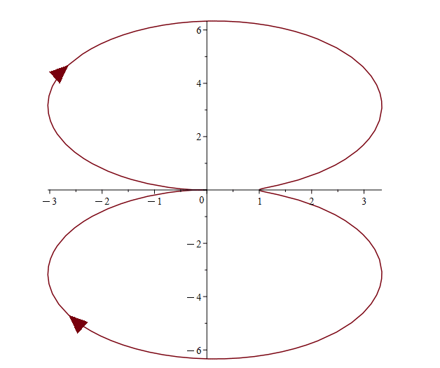

図3の輪っかの部分を拡大したものを図4に示します。
赤矢印で示したラインが「-1」より左側を通って虚軸のマイナス側へと入っていますね。この「-1」の右側か左側かで安定・不安定が分かれるのです。「-1」の上は安定限界なんて言われていますが、実質的にギリギリは何か変動があるとすぐに不安定になるので、「-1」より十分に右側を通過する方が安心です。
ちなみにナイキスト線図の安定判別はこの「-1」の右か左かが一番メジャーですが、ちゃんとナイキストの安定判別はもう少し条件があります。詳しく知りたかったら勉強してみてください。まぁ、でもほとんどこの「-1」の右か左かだけで判断できます。逆を言えばこれで不安定なら確実にダメですね。

最後にナイキスト線図で不安定となると、いったいどうなるのかを見ておきましょう。C1(s)とC2(s)のStep応答を図5と図6に示しています。安定な方は振動しながらも収束していってますね。逆に不安定な方は発散しています。
ナイキスト線図を使った安定判別を見ることでフォードバックシステムの安定性を簡単に予測できるところが、私がナイキスト線図をボード線図の次に使う利用なのです。


【English】
In my previous article, I discussed Bode plot, one of the frequency responses. In this article, I will introduce the Nyquist diagram, which I often use next to the Bode plot. There are many other frequency response diagrams, but Bode plots and Nyquist diagrams are sufficient for me. Everyone should study other frequency responses as needed.
What is a Nyquist diagram?
Some of you may be thinking, "Why can't I just use a Bode plot?" However, a Bode plot alone is sufficient to see the characteristics of the frequency domain.
You may be thinking, "Well, why do I need to see a Nyquist diagram? It is because there are some things that are useful with Nyquist diagrams.
In a very simple way, it is easy to see the stability of the feedback system in Figure 1: just by looking at the Nyquist diagram of the P(s)C(s) transfer function, we can get a good idea of the stability of the feedback system. The Nyquist diagram itself is explained in many books and online articles, so I will omit it in this article. However, with recent software (Maple in this article), you can type a single line of command and immediately get a Nyquist diagram. So let's get started and see how stable the feedback system is using Maple.
Let's look at the Nyquist diagram in Maple
The plant's system P(s) is as follows,
Let's take a look at the Nyquist plots for the following C1(s) and C2(s) controller systems, and since a Maple sample program is included at the end of this article, if you have Maple and take a look at the sample, you will see that the Nyquist diagrams can be displayed with a single line of the "NyquistPlot (sys)" command.
Figure 2 and Figure 3 show the Nyquist diagrams for the C1(s) and C2(s) controller systems displayed in Maple, respectively. The Nyquist diagrams for C1(s) and C2(s) are almost the same, with the only difference being that C2(s) has one loop in the negative part of the x-axis (real axis). In the Nyquist diagram, the x-axis is the real axis (Re) and the y-axis is the imaginary axis (Im).
This little loop is actually the dividing line between stable and unstable.
An enlargement of the loop in Figure 3 is shown in Figure 4.
The line indicated by the red arrow passes to the left of "-1" and enters the negative side of the imaginary axis. The right or left side of the "-1" is the difference between stable and unstable. The line passing through "-1" is said to be the limit of stability, but it is safer to pass well to the right of "-1" because it becomes unstable as soon as there is any fluctuation at the very edge of the line.
By the way, the most major stability discriminant of the Nyquist diagram is whether this "-1" is to the right or left of the "-1," but there are a few more conditions to properly discriminate Nyquist stability. If you want to know more details, please study. Well, but you can almost always tell whether it is to the right or left of this "-1". In other words, if it is unstable, it is definitely not good.
Finally, let's look at what happens when the Nyquist diagram becomes unstable: the Step responses of C1(s) and C2(s) are shown in Figures 6 and 7. The stable one is converging while oscillating. Conversely, the unstable one is diverging.
The fact that the stability of the Fordback system can be easily predicted by looking at the stability discrimination using the Nyquist diagram is the use I make of the Nyquist diagram next to the Bode plot.
【Sample】
Created by Maple 2023.2
この記事が気に入ったらサポートをしてみませんか?