
Mapleで制御工学の基礎虎の巻3「周波数応答(ボード線図)」

前回は記事では、一定の入力に対する応答であるステップ応答と瞬間的な外乱入力に対する応答であるインパルス応答について見てみました。今回は時間的に変化のある入力に対する対象とするシステムの応答を見てみたいと思います。とは言っても、入力に対する定義を全くしないで自由に変化する入力に対する応答を見るというのでは際限がないので、一般的には周波数別のSin波形に対するシステムの応答で評価します。簡単に言うと、Sin(ωt)のωを小さいもの(低周波)から大きいもの(高周波)まで変えたときに対象システムの出力がどうなるかを見ます。また、周波数応答はボード線図、ナイキスト線図、ニコルス線図など、さまざまなものが提案されています。今回は開発の場でもよく使われるボード線図について見てみたいと思います。
ボード線図とは?
先ほど述べたように対象とするシステムへの入力はSin波形であるSin(ωt)を入力とします。このSin波形の周波数であるωを小さいものから大きいものまで変化させたときの対象システムのゲインの大きさの変化(ゲイン線図)と位相の変化(位相線図)をそれぞれプロットした図がボード線図です。ゲイン線図は横軸を周波数(ω)とし、縦軸をゲイン線図はゲイン[dB]、位相線図も横軸は周波数(ω)とし、縦軸を進み位相(プラス)または遅れ位相(マイナス)の位相[deg]をプロットします。あとで説明しますが下方に記載してある図1のような図になります。
二次系の伝達関数
前回の記事まではバネマスダンパ系の伝達関数のパラメータ(重さやバネ定数やダンパ係数)を変化させたときの応答の様子を見てきましたが、今回は二次系の伝達関数を使って応答を見てみたいと思います。二次系の伝達関数の形式に当てはめると、システムの応答を簡単に解析できるので便利なので今回は紹介するために二次系の伝達関数を対象としました。
二次系の伝達関数は次式の形になります。この形の伝達関数は伝達関数のパラメータである固有角周波数ωと減衰比ζの値から応答を推測することができます。
ここでちょっとお詫びですが、多くの教科書ではこの固有角周波数はωn(nは下付き文字)を使って、入力のSin(ωt)のωと区別します。私の使っているMapleではωn(nは下付き文字)にすると数列と認識してしまいうまくできませんでした。そのため二次系の伝達関数の式の固有角周波数も入力の周波数であるωと同じ文字にしてしまっていますが、入力の周波数のωと二次系のωは全くの別物のωとご理解ください。
次の節でこの固有角周波数ωと減衰比ζを変化させたときのボード線図を見てみましょう。

ω:固有角周波数
ζ:減衰比
Mapleでボード線図を見てみよう
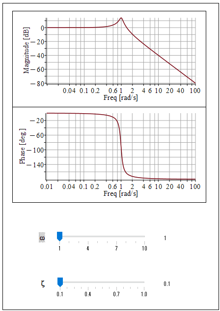
図1は二次系の伝達関数のωを図2はζを変化させたときのボード線図を表しています。先ず簡単にこのボード線図の解説すると、ゲイン線図(上側)は入力の周波数が大きくなるとピークを迎えてその後、右下がりになっています。ゲインがゼロより大きいピークを持っているので、ピークになる入力周波数の前後では入力よりも大きな出力になります。その後、右下がりにゼロを下回っていくので、入力周波数が大きくなっていくと出力が小さくなっていくます。要するに今回のシステムでは高周波ノイズのようなものは出力に現れないことがわかります。逆に高い周波数で動かそうとしても反応してくれないとも言えます。
位相線図(下側)も入力周波数が大きくなると右下がりになって-180[deg]に近づいていきます(-180[deg]にはならない)。これは入力の周波数が高くなってくると出力の位相が入力に対して遅れていくということです。
さて本題の二次系の固有角周波数ωを変化するとどうなるか図1を見てわかるとおり、ゲイン線図のピークや位相線図の遅れが大きくなっていく入力の周波数が変化していますね。固有角周波数ωの値ピークを迎える入力周波数であり位相が-90[deg]となります。ちなみに図2で減衰比ζを変化させているのでわかりますが、減衰比ζを大きくしていくとピークがなくなり、位相線図の傾きが緩やかになります。固有角周波数ωはピークの位置と言いましたがピークのない場合にはゲイン線図のおおよそ下がり始める位置になります。


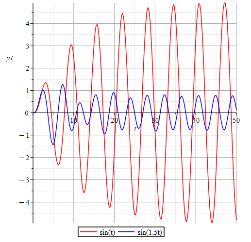
次に固有角周波数ω=1、減衰比ζ=0.1とした場合を例に入力の周波数を変えたときの出力応答を見てみましょう。図3に固有角周波数ω=1、減衰比ζ=0.1としたときのボード線図を示し、図4にそのシステムに対して入力をsin(t)とした場合とsin(1.5t)とした場合の出力の様子を示しています。
ゲイン線図のピークを迎える1[rad/s]となるsin(t)を入力にすると入力の振幅「1」より大きい値になっていますね。逆にゲイン線図で0[dB]を下回る入力周波数である1.5[rad/s]としたsin(1.5t)の入力では入力の振幅「1」より小さい値になっていますね。さらに入力周波数が大きくなっていくほど出力には現れなくなっていきます。
Mapleのサンプルワークシートをこの記事の終わりにつけてありますので、Mapleをお持ちの方は固有角周波数ωや減衰比ζを変えてみたり、実際に入力周波数を変えてみて出力の変化を見てみると理解が増すことでしょう。
【参考】二次系のステップ応答
二次系の伝達関数のボード線図を見てきましたが、固有角周波数ωや減衰比ζを変えたときのステップ応答はどうなるのかも見ておきましょう。
図5は二次系の伝達関数のωを図6はζを変化させたときのステップ応答を表しています。
固有角周波数ωが大きくなると振動の周波数が大きくなっていることがわかります。実は山の数は変わっていないので、ぎゅっと短い時間で収束するように押し込んでいるようなイメージですね。
減衰比ζを見てみましょう。まさに減衰比の名に相応しく、減衰比が大きくなると振動しなくなっているのがわかります。

ゲイン余裕と位相余裕
ボード線図でもう一つ大事なのがシステムの安定性の指標の1つであるゲイン余裕と位相余裕です。システムのバラつきも入力誤差も全くないようなシステムであれば安定余裕(ゲイン余裕や位相余裕)はゼロでもよいかもしれません(なお、マイナスだと不安定です)が、そんなことまずありませんからある程度の安定余裕を持つ必要があります。経験的な安定余裕の目安は以下です。書籍によって多少さはあるもののだいたい似た数字だと思います。
ゲイン余裕と位相余裕の経験的な目安
ゲイン余裕 10[dB]以上
位相余裕 45[deg]以上
それではボード線図から対象とするシステムの安定余裕を見てみましょう。
ゲイン余裕
位相線図で-180[deg]になる入力周波数でのゲイン線図のゲインの値から0[dB]までの差です。例えばゲイン線図の読みが-20[dB]ならゲイン余裕は20[dB]となります。読みの値とゲイン余裕の値の符号が逆になることに注意してください。絶対値ではありませんので、ゲイン線図の読みが20[dB]なゲイン余裕は逆にマイナスになり不安定となります。
位相余裕
ゲイン線図でゼロを下回る入力周波数での位相線図の位相の値の-180[deg]を基準とした位相の値です。例えば-100[deg]だとすると-180[deg]より80[deg]大きいので位相余裕は80[deg]となります。-180[deg]より下になると不安定となります。
それでは実際にボード線図からゲイン余裕と位相余裕を見てみましょう。
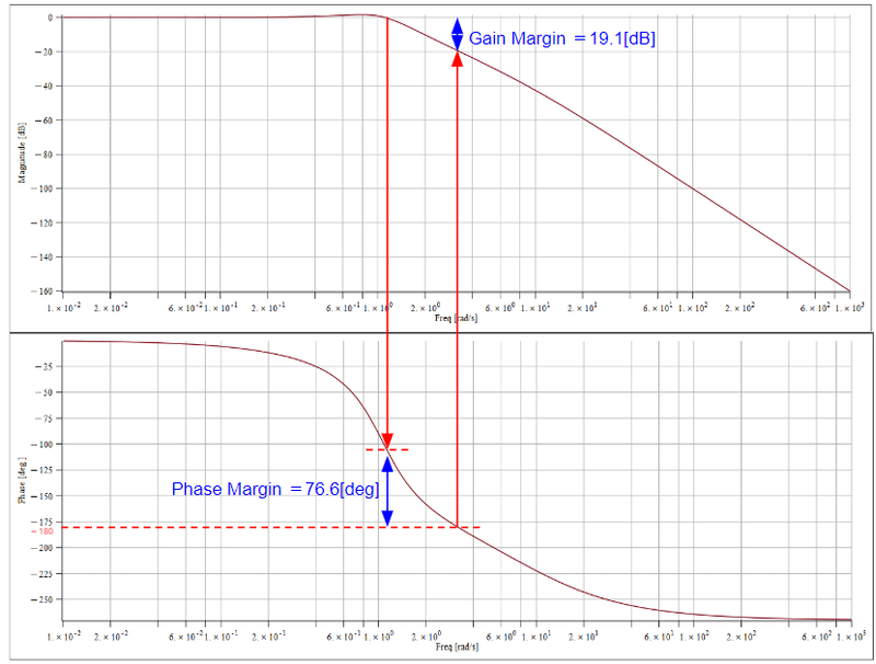
二次系では位相線図が-180[deg]を下回らないため、今回は以下の3次の伝達関数を例に見てみましょう。この伝達関数のボード線図を図7に示します。

図7を見ると位相線図で-180[deg]になる入力周波数でのゲインは約-19.1[dB]ですので、ゲイン余裕は19.1[dB]となります。
次に位相余裕ですが、ゲイン線図で0[dB]を下回る入力周波数での位相は約-103.4[deg]なので位相余裕は76.6[deg]となります。
今回も見た伝達関数のゲイン余裕も位相余裕も目安の値を満足しているので安定したシステムと言えます。
じゃぁゲイン余裕、位相余裕があれば何がいいの?
簡単に言えば、ゲイン余裕や位相余裕があれば、入力ゲインをまだ大きくすることができるってことです。ゲインを大きくするとゲイン線図(ボード線図の上側の線図)が上方にオフセットしていきます。そうするとゲイン線図がゼロを下回る位置が右側に移動するので、一般的なゲイン線図も位相線図も右下がりの場合には、ゲイン線図がゼロになる周波数に対応する位相もさらに遅れる側になるため、位相余裕は減少しますし、位相が-180[deg]に対応するゲインも上昇するためゲイン余裕も小さくなっていきますよね。余裕が小さくなるとちょっとした外乱でも安定余裕を超えて不安定に、簡単に言えば変な応答や望ましくない応答になってしまうかもしれません。そんためにちょっとやそっとの外乱でも不安定にならないように安定余裕(ゲイン余裕と位相余裕)をある程度持つようなシステムにしなければならないのです。
【English】
In the previous article, we looked at step response, which is the response to a constant input, and impulse response, which is the response to an instantaneous disturbance. In this article, we will look at the response of the target system to a time-varying input. However, since there is no limit to looking at the response to a freely varying input without defining the input at all, we will generally evaluate the system's response to a sine waveform at various frequencies. Briefly, it looks at what happens to the output of the target system when the ω of Sin(ωt) is changed from small (low frequency) to large (high frequency). Various frequency responses have also been proposed, including Bode plot, Nyquist plot, and Nichols chart. In this article, we will look at Bode plot, which are often used in development.
What's a Bode plot?
As mentioned earlier, the input to the target system is a Sine waveform, Sin(ωt). The Bode diagram plots the change in gain magnitude (Magunitude plot) and phase change (Phase plot) of the target system when the frequency of this Sine waveform, ω, is changed from small to large. For the Magunitude plot, the horizontal axis is frequency (ω) and the vertical axis is Magunitude [dB] for the Magunitude plot, and for the Phase plot, the horizontal axis is frequency (ω) and the vertical axis is Phase [deg] for the advance phase (positive) or delay phase (negative) is plotted. The figure will look like Figure 1 shown below, which will be explained later.
Transfer function of Second-order system
In the previous article, we looked at the response of a spring-mass damper system when the transfer function parameters (weight, spring constant, and damper coefficient) are varied, and now we would like to look at the response using the transfer function of a second-order system. We have targeted the transfer function of a second-order system for the purpose of this introduction because it is useful to easily analyze the response of a system by applying the transfer function form of a second-order system.
The transfer function of a second-order system takes the form of the following equation. The response of a transfer function of this form can be inferred from the values of the transfer function parameters, natural angular frequency ω and damping ratio ζ.
A little apology here, but most textbooks use ωn (n is a subscript) for this natural angular frequency to distinguish it from ω in the input Sin(ωt). In my Maple, it is recognized as a number sequence when ωn (n is a subscript) is used, and I could not get it to work. Therefore, the natural angular frequency of the transfer function of the second-order system is also set to the same letter as the input frequency, ω. Please understand that the input frequency, ω, and the second-order system, ω, are two completely different things, ω.
Let us look at the Bode plot when this natural angular frequency ω and damping ratio ζ are varied in the next section.
ω:Natural angular frequency
ζ:Damping ratio
Let's look at the Bode plot in Maple
Figure 1 shows the Bode plot of the transfer function ω for a second-order system, and Figure 2 shows the Bode plot when ζ is varied. First, a brief explanation of this Bode plot is that the Magunitude plot (upper side) peaks as the input frequency increases and then declines to the right. Since the gain has a peak greater than zero, the output is greater than the input before and after the peak input frequency. After that, the gain falls to the right below zero, so the output becomes smaller as the input frequency increases. In short, in this system, you can see that nothing like high-frequency noise appears in the output. Conversely, it can be said that the system does not respond to input at high frequencies.
The phase plot (lower side) also declines to the right and approaches -180[deg] (not -180[deg]) as the input frequency increases. This means that as the input frequency increases, the output phase lags behind the input.
As you can see in Figure 1, the frequency of the input that causes the peak of the Magnitude plot and the delay of the Phase plot to increase changes as you change the natural angular frequency ω of the second-order system. This is the input frequency at which the value of natural angular frequency ω peaks and the phase is -90[deg]. Incidentally, as you can see from the change in damping ratio ζ in Figure 2, as you increase the damping ratio ζ, the peak disappears and the slope of the phase plot becomes more gradual. The natural angular frequency ω is said to be the position of the peak, but if there is no peak, it is the approximate position where the magnitude plot begins to fall.
Next, let us take the case where the natural angular frequency ω = 1 and the damping ratio ζ = 0.1 as an example to see the output response when the input frequency is changed. Figure 3 shows the Bode plot when natural angular frequency ω = 1 and damping ratio ζ = 0.1, and Figure 4 shows the output response when the input is sin(t) and sin(1.5t) for that system.
If the input is sin(t), which is 1[rad/s], the peak of the Magunitude plot, the output is greater than the input amplitude "1", right? Conversely, for the input sin(1.5t) with an input frequency of 1.5[rad/s], which is below 0[dB] in the Magunitude plot, the output is smaller than the input amplitude "1," right? Further, the larger the input frequency, the less it appears in the output.
A sample worksheet for Maple is included at the end of this article. If you have Maple, you can try changing the natural angular frequency ω and damping ratio ζ, or actually change the input frequency and see how the output changes to gain a better understanding.
【Supplementary information】 Step response of second-order system
Above we have seen the Bode plot of the transfer function of a second-order system, but now let us also see what happens to the step response when the natural angular frequency ω and damping ratio ζ are changed. Figure 5 shows the step response of the transfer function of the second-order system when ω is varied and Figure 6 shows the step response when ζ is varied.
We can see that as the natural angular frequency ω increases, the frequency of the vibration is increasing. In fact, the number of peaks has not changed, so the waveform looks as if it is being pushed to convergence in a squeezed and short time.
Let's take a look at the damping ratio ζ. As the damping ratio increases, the output waveform no longer oscillates.
Gain Margin and Phase Margin
Another important factor in Bode plot is the Gain Margin and Phase Margin, which are one of the indicators of stability of the system. If the system is such that there is no system deviation or input error at all, zero stability margin ( Gain Margin and Phase Margin) may be acceptable (negative values are unstable), but this is rarely the case, so it is necessary to have a certain stability margin. The following is a rough guideline of the stability margin based on our experience. The figures may vary from book to book, but they are generally similar.
An Empirical Guideline for Gain Margin and Phase Margin
Gain Margin 10[dB] or more
Phase Margin 45[deg] or more
Then, let's take a look at the stability margin of the target system from the Bode plot.
Gain Margin
It is the difference from the gain value on the Magunitude plot to 0[dB] at the input frequency that is -180[deg] on the Phase plot. For example, if the Magunitude plot indicates a reading of -20[dB], the Gain Margin is 20[dB]. Note that the sign of the reading and the Gain Margin value are reversed. Since this is not an absolute value, a Gain Margin of 20[dB] in the Magunitude plot reading will conversely be negative and unstable.
Phase Margin
This is the phase value based on -180[deg] of the phase value in the Phase plot at the input frequency below zero in the Magunitude plot. For example, if -100[deg] is 80[deg] greater than -180[deg], the phase margin is 80[deg]. If it becomes lower than -180[deg], it becomes unstable.
Now let's actually look at the Gain Margin and Phase Margin from the Bode plot. Since the phase plot never falls below -180[deg] in a second-order system, let us look at the following third-order transfer function as an example this time. The Bode plot of this transfer function is shown in Figure 7.
Figure 7 shows that the gain at the input frequency that is -180[deg] in the Phase plot is about -19.1[dB], so the gain margin is 19.1[dB].
Next is the Phase Margin. The phase at the input frequency below 0[dB] in the Magunitude plot is about -103.4[deg], so the Phase Margin is 76.6[deg].
The Gain Margin and Phase Margin of the transfer function that we have seen again satisfy the guideline values, so we can say that the system is stable.
So what are the benefits of having Gain Margin & Phase Margin?
Simply saying, it means that the input gain can still be increased if there is enough Gain Margin or Phase Margin. As the gain is increased, the gain Magunitude plot (the upper side of the Bode plot) is offset upward. The position at which the Magunitude plot falls below zero moves to the right, and since the Gain and Phase plots generally show that both gain and phase decrease as the frequency increases, the phase corresponding to the frequency at which the Gain plot falls to zero moves further to the slow side, and the Phase Margin also decreases. Therefore, the gain corresponding to a phase of -180[deg] also increases, and the Gain Margin also decreases. If the margin becomes small, even a slight disturbance may exceed the stability margin and cause instability, or simply put, a strange or undesirable response. For this reason, the system must have a certain amount of stability margin (Gain Margin and Phase Margin) so that even a slight disturbance will not cause instability.
【Sample】
Created by Maple 2023.2
この記事が気に入ったらサポートをしてみませんか?