
Mapleで制御工学の基礎虎の巻2「ステップ応答とインパルス応答」

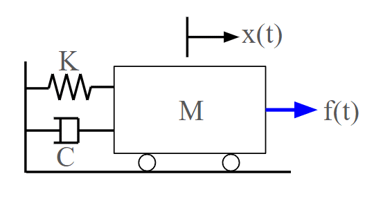
本記事では『Mapleで制御工学の基礎虎の巻1「ラプラス変換」』の記事で導いた図1のバネマスダンパ系の伝達関数のステップ応答やインパルス応答をMapleを使って見ていこうと思います。
なお、本記事で紹介するMapleの例は記事の最後にサンプルとして添付してあります。Mapleをお持ちの方はダウンロードして参考にしてみてください。
ステップ応答
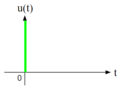
図1のシステムへの入力f(t)に図2のステップ状の入力を与えたときの出力、図1の場合x(t)の応答がステップ応答です。ステップ応答はステップ状の入力への追従性を見るためのものになります。

Mapleでステップ応答を見てみよう
次の「Mapleコマンド1」ようにMapleのワークシートに記入します。
1行目はステップ応答のコマンドを使うために記載します。
2行目から4行目は伝達関数のパラメータの値を入力しています。
この値をデフォルトの値として、それぞれの値を変えてみて、ステップ応答の変化を見てみましょう。
「Mapleコマンド2」に記載したように、Mの値を変えてみましょう。
M1からM3までの値を設定して、「TransferFunction」コマンドで、それぞれの伝達関数をsys1からsys3として設定します。

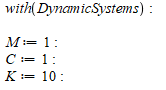
「Mapleコマンド3」に記載したようにコマンドを記入すると、sys1からsys3の伝達関数のステップ応答が表示されます(図3)。重さであるMの値が大きくなるほど応答がゆっくりになり、一方で振動の減衰がしにくくなっていますね。

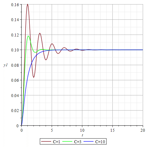
同様に今度はダンパ抵抗のCを変えて見てみましょう(図4)。ダンパ抵抗Cが大きくなるほど振動しなくなっています。しかし、その背反として応答が遅くなっていますね。
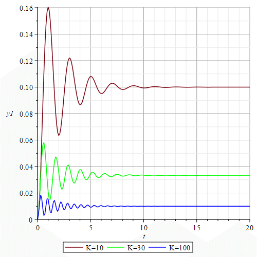
最後にバネ定数のKを変えてみましょう(図5)。バネ定数が大きくなるとバネの力が大きくなるために変位が小さくなりますが、振動の周波数も高くなっていますね。
以上のようにステップ応答を見ることによって応答の速さや、オーバーシュートの大きさ、振動の様子を知ることができます。制御を付加することで理想的な振る舞いにシステムをコントロールしていく上で、最初に見るとよい応答性能だと思います。
パラメータをもっと簡単に動かしながら応答を見てみたい
「Mapleコマンド4」のようにコマンドを記述すると図6のようにスライダーを動かして応答を見ることができます。


インパルス応答
ステップ応答では図2のステップ状の入力を与えたましたが、インパルス応答は図7に示すインパルス入力をシステムに与えて、そのときの応答を見ます。ステップ応答が入力への追従性を見るのに対して、インパルス応答はシステムへの入力外乱の影響を見るものになります。
Mapleでインパルス応答を見てみよう
次の「Mapleコマンド5」ようにMapleのワークシートに記入します。
なお、ステップ応答のワークシートと同じワークシートに記載する場合には「with(DynamicSystems):」のコマンドはすでに記載してあるので、改めて記載する必要はありません。もしステップ応答のワークシートと分けてワークシートを新しくする場合には「with(DynamicSystems):」のコマンドを最初に記載するようにしてください。インパルス応答のコマンドを使うために必要なコマンドです。

「Mapleコマンド5」に記載したようにコマンドを記入して実行すると図8のようにインパルス応答が見れます。ステップ応答と同様にsys1からsys3の伝達関数のインパルス応答が表示されています(図8)。重さであるMの値が大きくなるほど、インパルス入力の影響は出にくい、要するにピークが立ちにくくなっていますが、振動の減衰がしにくくなっていますね。

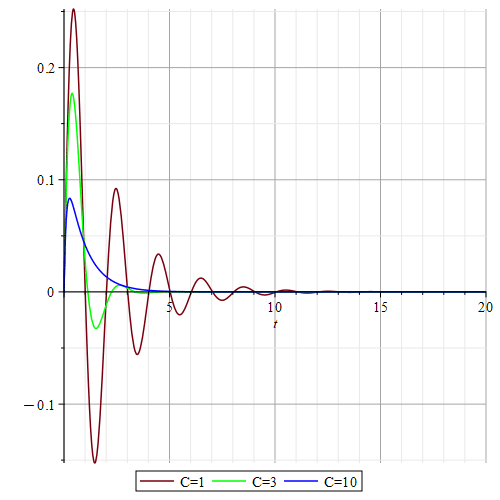
同様に今度はダンパ抵抗のCを変えて見てみましょう(図9)。ダンパ抵抗Cが大きくなるほど入力外乱の影響が少なくなっていますね。
バネ定数のKも変えてみましょう(図10)。バネ定数が大きくなるとインパルス入力による振幅の変化は抑えられていますし、減衰も早めですが、振動数も高くなってしまっています。

以上のようにインパルス応答を見ることによってシステムへのインパルス入力外乱の影響を見ることができます。制御設計をする際には、目標への追従性能だけでなく、外乱による影響も考えていかなければなりません。
今回紹介したステップ応答とインパルス応答はシステムを制御する上で知っておくべき応答の基本の1つです。目的に応じて見ておくべき応答はいろいろありますので、みなさんの目的に応じていろいろな応答性能を見てみてください。
パラメータをもっと簡単に動かしながら応答を見てみたい
ステップ応答と同じようにインパルス応答もスライダーを動かして応答を見ることができます。「Mapleコマンド6」のようにコマンドを記述すると図11のようにスライダーでパラメータを変えることができます。

【English】
In this article, we will use Maple to look at the step response and impulse response of the transfer function of the spring-mass damper system shown in Figure 1, which was derived in the article "Laplace Transform" in "Basic Control Engineering with Maple Volume 1". The Maple example introduced in this article is attached as a sample at the end of this article, so if you have Maple, please download it and refer to it.
Step Response
The step response is the response of the output, x(t) in the case of Figure 1, when a step-shaped input is given to the system f(t) in Figure 2. The step response is used to see how well the system follows the step input.
Let's look at the Step Response in Maple
Fill in the Maple worksheet as in the following "Maple command 1".
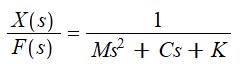
The first line is written to use the step response command; the second through fourth lines are for entering the values of the transfer function parameters. Using these values as default values, try changing each value and see how the step response changes.
Let's change the value of M as described in "Maple Command 2," setting the values from M1 to M3 and then using the "TransferFunction" command to set each transfer function as sys1 through sys3.
Filling in the commands as described in "Maple Command 3," the step response of the transfer function from sys1 to sys3 is displayed (Figure 3). The larger the value of M, the weight, the slower the response becomes, while the vibration is harder to damp.
Similarly, let us now change the damper resistance C (Figure 4). The larger the damper resistance C, the less it vibrates. On the other hand, the response is slower.
Finally, let's change the spring constant K (Figure 5). As the spring constant increases, the displacement is smaller because the spring force is greater, but the frequency of vibration is higher.
By looking at the step response as described above, we can see how fast the response is, how large the overshoot is, and how the system oscillates. It is a good first look at the response performance in controlling the system to the ideal behavior by adding control.
Let's see the response while moving the parameters easily
If you write a command like "Maple command 4," you can move the slider to see the response as shown in Figure 6.
Impulse Response
While the step response was given a step input as shown in Figure 2, the impulse response is given an impulse input as shown in Figure 7, and then the response is observed. While the step response looks at how well the system follows the input, the impulse response looks at the effect of the input disturbance on the system.
Let's look at the Impulse Response in Maple
Fill in the Maple worksheet as in the following "Maple command 5." If you are entering the command in the same worksheet as the step response worksheet, the "with(DynamicSystems):" command has already been entered, so there is no need to enter it again. If you are creating a new worksheet that is separate from the step response worksheet, the "with(DynamicSystems):" command should be placed first. This command is required to use the impulse response commands.
When the command is filled in and executed as described in "Maple Command 5," the impulse response can be viewed as shown in Figure 8. Similar to the step response, the impulse response of the transfer function from sys1 to sys3 is displayed ( Figure 8 ). The larger the value of M, which is the weight, the harder it is for the impulse input to have an effect, in other words, the harder it is for the peak to rise, but the harder it is for the vibration to be damped.
Similarly, now let's look at the damper resistance C differently (Figure 9). The larger the damper resistance C, the less the effect of the input disturbance.
Let's also change the spring constant K (Figure 10). As the spring constant increases, the amplitude change due to impulse input is suppressed and damping is faster, but the frequency is also higher.
By looking at the impulse response as described above, we can see the effects of impulse input disturbances on the system. When designing control, we must consider not only the performance of following the target, but also the effects of disturbances. The step response and impulse response introduced here are one of the basics of response that should be known when controlling a system. There are various types of response that should be looked at for different purposes, so please take a look at various types of response performance according to your own objectives.
Let's see the response while moving the parameters easily
As with the step response, the impulse response can be viewed by moving the slider. If you write a command like "Maple command 6," you can use the slider to change the parameters as shown in Figure 11.
【Sample】
Created by Maple 2023.2
この記事が気に入ったらサポートをしてみませんか?