
MapleSimで超簡単な油圧モデルを作ってみた#4(方向切り替えバルブでシリンダを動かしてみる)

前回までにポンプの流量を分配したり、回路圧が高まった時にリリーフさせて回路の安全を保つ回路をモデル化してきました。今回はこれまでのモデルを応用して方向制御バルブを可変オリフィスを使って作成し、さらにシリンダブロックを設置してシリンダを動かしてみます。
作成する油圧回路
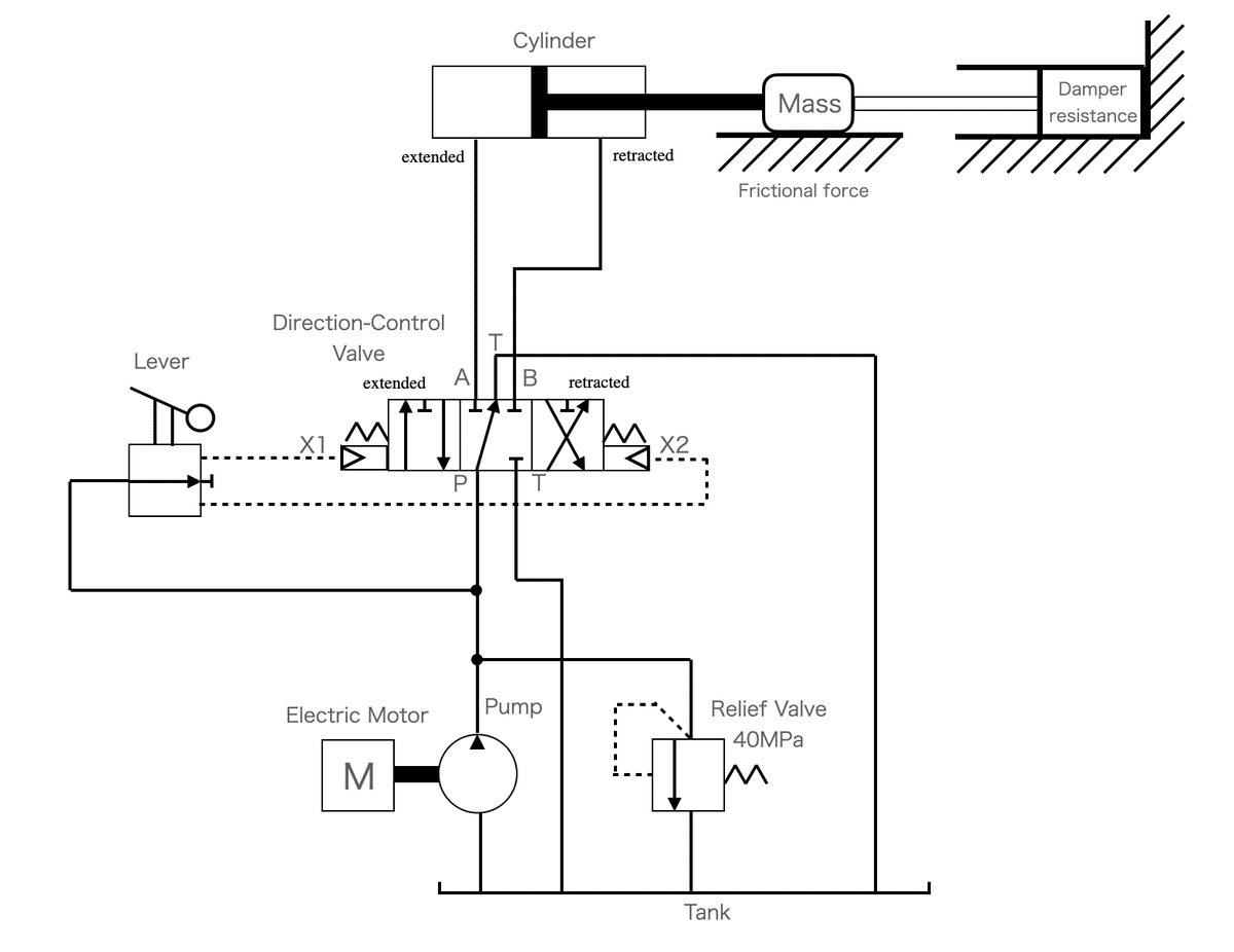
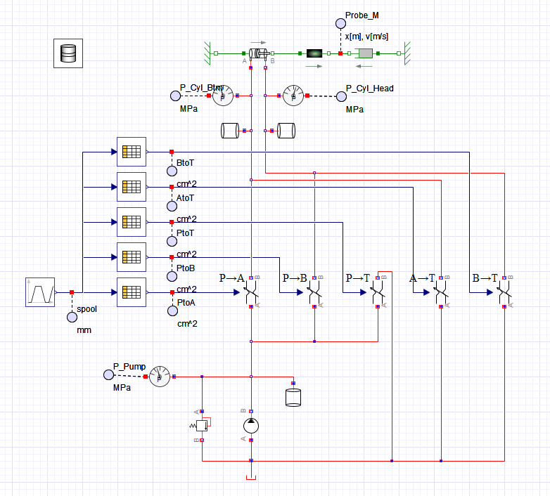
今回作成する油圧回路は図1の回路です。
レバーによってバルブを切り替えることでシリンダを伸ばしたり、縮めたりします。図1の方向切替バルブの絵を見ると、「伸び」「中立」「縮み」の3つポジションが描かれています。カチカチとデジタル的に3つの状態が切り替わるバルブもありますが、今回作成するバルブはリニアに変化するようにします。要するに中立と伸びの中間のポジションも取れるようにします。それは何のためかと言うと、タンクへ戻るラインとシリンダへ行くラインの2つの開口面積バランスでシリンダへ送る流量を調整することができるからです。これによって、レバーの操作量によってシリンダのスピードを制御できるようになるのです。
バルブ部分のモデル化
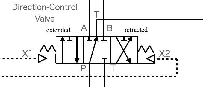
バルブの部分をもう少し詳しく見てみましょう。図2のバルブ部分の拡大図を見ると、5つのラインを確認できます。
・P(ポンプ) →A(シリンダボトム)
・P(ポンプ) →B(シリンダヘッド)
・P(ポンプ) →T(タンク)
・A(シリンダボトム) →T(タンク)
・B(シリンダヘッド) →T(タンク)
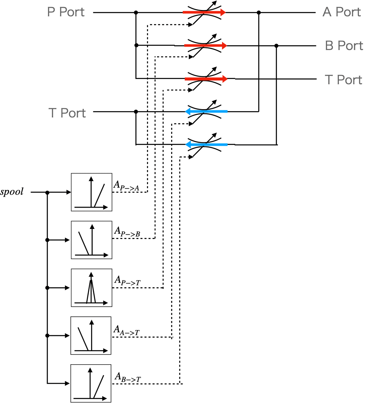
したがって、図3に示す5つの可変オリフィスでモデル化できることになります。なお、タンクへは2つのポートがつながっていることになります。
それではMapleSimでバルブをモデル化してみましょう。
前回作成したモデルをベースに改造していきますので、ポンプやリリーフバルブ、可変オリフィス、作動油の設定については過去の記事を参照してください。
前回作成したモデルのポンプやリリーフバルブ、チャンバーはそのまま使います。ポンプの容量だけ、100[L/min]から50[L/min]に変更します。
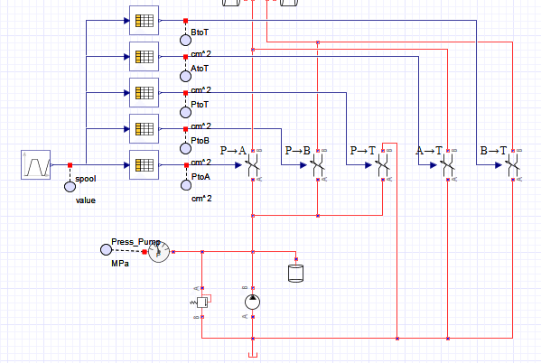
図4に示すように、ポンプの出力に5つの可変オリフィスを配置してつなげます。それぞれのオリフィスには一次元補間を行う「Lookup Table 1D」ブロックを配置してつなげます。さらに可変オリフィスの開口面積を制御するspoolの時系列信号を作るため、「Trapezoid」ブロックを配置して5つの「Lookup Table 1D」ブロックにつなげます。また、spoolの値と各可変オリフィスの開口面積(「Lookup Table 1D」ブロックの出力値)を見たいのでprobeを付けておきます。
また、タンクポートに連結される可変オリフィスは図4に示すようにタンクブロックに連結します。
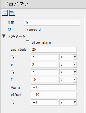
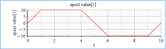
spoolの時系列信号を作る「Trapezoid」ブロックの設定を図5に示します。正しく設定すると図6のような出力結果になります。これによってスプールが中立の位置からシリンダを伸ばすプラス側、シリンダを縮ませるマイナス側に動き、シリンダの伸縮をシミュレーションするバルブ指令を作ることができました。
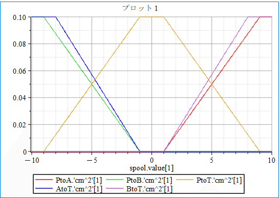
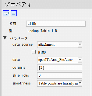
次に可変オリフィスの設定をします。図7にspool位置に対する各可変オリフィスの開口面積を示します。5つの可変オリフィスがありますから、5つのcsvファイルを作成して、図8のように各可変オリフィスに対応する「Lookup Table 1D」にセットします。「Lookup Table 1Dの使い方」を参照してください。図8はPからAの設定例ですので、それぞれの可変オリフィスに対応したcsvファイルを「Lookup Table 1D」の設定にセットしてください。
シリンダブロックを設置
次にシリンダブロックを含む伸縮機構部分を作成します。
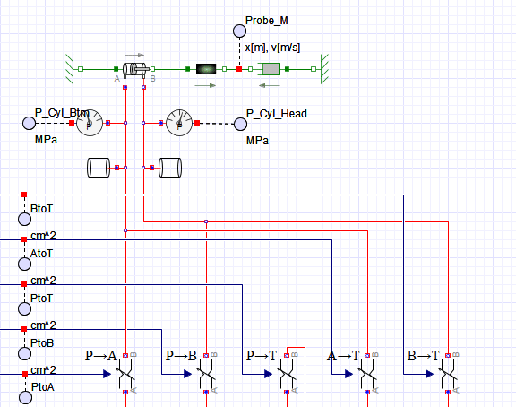
図9に示すようにシリンダブロックを設置し、さらにシリンダのロッドの先にMassブロック(慣性)、さらにその先にダンパーブロックを設置してそれぞれを連結します。シリンダのボトム側とダンパーのMassブロックがつながっていない側には動きを固定する「Translational Fixed」ブロックを設置してつなげます。
シリンダのAポート(ボトム側)とBポート(ヘッド側)には図9に示すように各可変オリフィスのAポート、Bポートと連結する可変オリフィスとつなっげます。
さらにAポートとBポートにはチャンバーを設置してつなげます。AポートとBポートのチャンバー容積は0.0001[m^3]と設定します。また、AポートとBポートの圧力を測定したいので、圧力センサを設置してprobeで見れるようにしておきます。
次に各ブロックの設定をします。
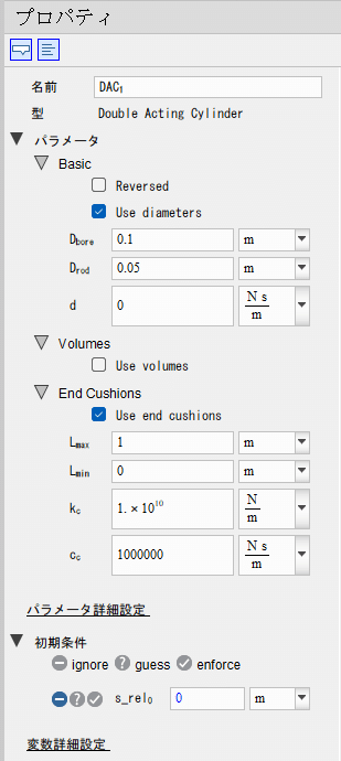
シリンダの設定を図10に示します。シリンダの特性値としてボア径(ボトム側の内径)とロッド径で設定できるように「Use diameter」にチェックを入れます。ボア径とロッド径にはそれぞれ0.1[m]、0.05[m]をセットします。
あと、シリンダの伸縮の長さを設定するために「Use end cushions」にチェックを入れて、シリンダの最大長さLmaxを1にしておきます。これでシリンダは1[m]伸びて、それ以上は伸びないようになります。シリンダのストロークエンドで止めるための抗力の設定をKcとCcでしますが、止まらないとか、振動するとかない限りデフォルトのままにしておきます。
その他もとりあえずデフォルトの値にしておきます。
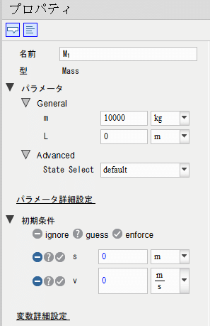
Massブロックの設定をします。
重さm(慣性)を10000[kg]に設定します。
その他はデフォルトのままにします。
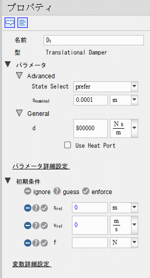
ダンパーブロックの設定をします。
ダンパーブロックのダンパ抵抗dは800000[Ns/m]にします。
その他はデフォルトのままにします。
以上でモデル化は完了です。
作り上げたモデルの全体を図13に示します。
シミュレーション実行
それでは実行ボタン「▶️」を押してシミュレーションをしてみましょう。
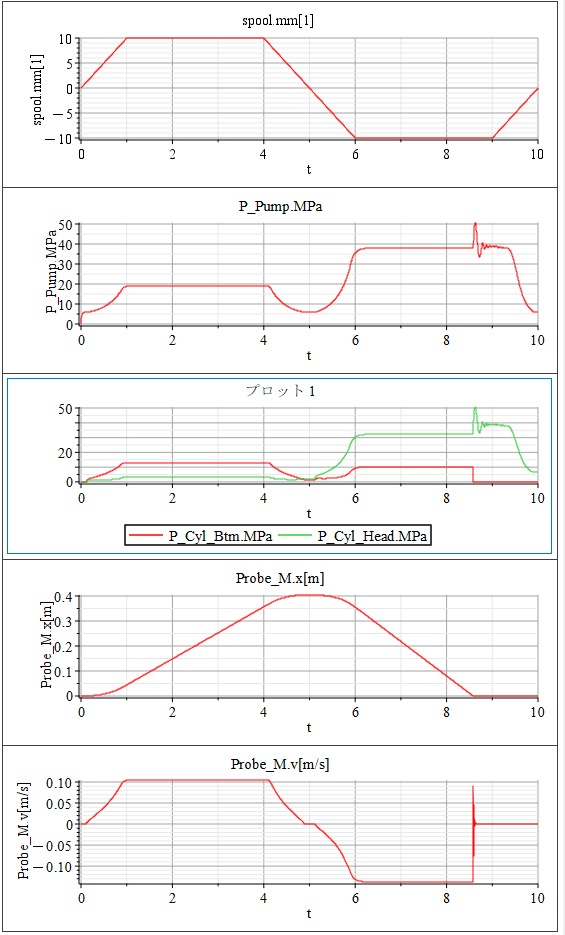
シミュレーション結果を図14に示します。
シリンダが伸縮しているのがわかります。
伸びに比べて縮みが速いのはシリンダの面積比が違うからです。ポンプの50[L/min]一定で吐き出しているので、ロッドの分だけシリンダのヘッド側は面積が小さいため、同じ流量で動かすと縮み側が速く動くのです。速度が速い分、ダンパ抵抗が大きくなっポンプ圧が大きくなっています。
【English】
Previously, I have modeled a circuit that distributes the flow rate of a pump and relieves it when the circuit pressure increases to keep the circuit safe. This time, I will apply the previous models to create a directional valve using a variable orifice, and then install a cylinder block to move the cylinder.
Hydraulic Circuit to be created
The hydraulic circuit to be created is shown in Figure 1. The cylinder is extended or retracted by switching the valve with a lever. The picture of the direction-control valve in Figure 1 shows three positions: "extended," "neutral," and "retracted. Although there are valves that digitally switch between the three states, the valve we are creating this time will also be able to take a position between neutral and extended (contracted). The reason for this is that the flow rate to the cylinder can be adjusted by balancing the opening area of the line returning to the tank and the line going to the cylinder. This allows the speed of the cylinder to be controlled by the amount of lever operation.
Modeling of Valve Section
Let's take a closer look at the valve section. Looking at the enlarged view of the valve section in Figure 2, we can see five lines.
・P (pump) → A (cylinder bottom),
・P (pump) → B (cylinder head),
・P (pump) → T (tank)
・A (cylinder bottom) → T (tank)・
・B (cylinder head) → T (tank).
Thus, it can be modeled with the five variable orifices shown in Figure 3. Note that two ports are connected to the tank.
Now let's model the valve in MapleSim.
We will modify the model based on the previously created model, so please refer to the previous articles for the pump, relief valve, variable orifice, and hydraulic fluid settings. The pump, relief valve, and chamber of the previously created model will be used as is. Only the pump capacity will be changed from 100[L/min] to 50[L/min].
As shown in Figure 4, five variable orifices are placed at the output of the pump and connected. Each orifice is connected to a "Lookup Table 1D" block that performs one-dimensional interpolation. In addition, a "Trapezoid" block is placed and connected to the five "Lookup Table 1D" blocks to create a time series signal for the spool that controls the opening area of the variable orifice. We also want to see the value of spool and the opening area of each variable orifice (the output value of the "Lookup Table 1D" block), so we add a "probe" block. The variable orifice connected to the tank port should be connected to the tank block as shown in Figure 4.
The settings for the "Trapezoid" block, which creates the time series signal for the spool, are shown in Figure 5. When set correctly, the output result is as shown in Figure 6. This allowed us to create a valve command that simulates cylinder expansion and contraction by moving the spool from the neutral position to the positive side to extend the cylinder and to the negative side to contract the cylinder.
Next, set up the variable orifices. Figure 7 shows the opening area of each variable orifice in relation to the spool position. since there are 5 variable orifices, create 5 csv files and set them to "Lookup Table 1D" corresponding to each variable orifice as shown in Figure 8. Refer to "How to Use Lookup Table 1D." Figure 8 is an example of settings from P to A. Set the csv files corresponding to each variable orifice to the "Lookup Table 1D" settings.
Addition of Cylinder
Next, the telescopic mechanism part including the cylinder block is created. As shown in Figure 9, a cylinder block is installed, a mass block (inertia) is added at the end of the cylinder rod, and a damper block is placed at the end of the cylinder rod and connected to each of them. The bottom side of the cylinder and the side of the damper not connected to the Mass block are connected by a "Translational Fixed" block that fixes the movement. The A port (bottom side) and B port (head side) of the cylinder are connected to variable orifices that are connected to the A and B ports of each variable orifice as shown in Figure 9. The chamber volumes of the A and B ports are set to 0.0001[m^3]. We also want to measure the pressure at the A and B ports, so a pressure sensor should be placed so that we can see the pressure in the probe.
Next, set up each block. Figure 10 shows the settings for the cylinder. Check the "Use diameter" check box so that the bore diameter (inside diameter of the bottom side) and rod diameter can be set as the cylinder's characteristic values. Set 0.1[m] and 0.05[m] for the bore diameter and rod diameter, respectively. Also, check "Use end cushions" to set the length of cylinder expansion and contraction, and set the maximum length of the cylinder, Lmax, to 1. This will cause the cylinder to extend 1[m] and no more. Kc and Cc are used to set the drag force to stop the cylinder at the end of its stroke, but unless the cylinder does not stop or vibrates, leave them at their default values. Other settings should be left at default values for the time being.
The Mass block is set up. Set the weight m (inertia) to 10000[kg]. Leave the other settings as default.
The damper block is set up. Set the damper resistance d of the damper block to 800000 [Ns/m]. Leave the other settings as default.
The modeling is now complete. The entire model we have created is shown in Figure 13.
Simulation
Now let's run the simulation by pressing the Run button "▶️". The simulation results are shown in Figure 14. You can see that the cylinder is expanding and contracting. The reason the cylinder is contracting faster than it is expanding is that the area ratio of the cylinder is different. Since the pump is discharging at a constant 50[L/min], the head side of the cylinder has a smaller area than the rod side, so the cylinder moves faster on the side that contracts if it is moved at the same flow rate. The faster speed results in greater damper resistance and therefore greater pump pressure.
【Sample Model】
Created by MapleSim 2023
この記事が気に入ったらサポートをしてみませんか?