MapleSimでLookup Table 1Dの使い方

モデル化でよく使う補間計算のMapleSimでの使い方について紹介します。
特によく使う一次元補間（Lookup Table 1D）について紹介します。

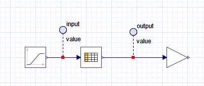
図1に「Lookup Table 1D」ブロックとそれを計算結果を見るための入力としてランプ入力と、出力のプローブを付けるために「Lookup Table 1D」ブロックの後ろにゲインブロックをダミーで付けています。

図1　Lookup Table 1Dブロック

「Lookup Table 1D」ブロックの補間テーブルをcsvファイルで作ります。
今回の例を図2に示します。

図2　csvファイル

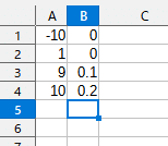
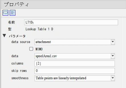
図3に「Lookup Table 1D」ブロックの設定を示します。
デフォルトの状態から変えるところは、「data source」と「data」だけです。
「data source」を「attachment」に設定します。
次に「data」を作成したcsvファイルを選択します。
それで設定は終わりです。シミュレーションを実行すると図4のような結果になります。

図3　「Lookup Table 1D」ブロックの設定

図4　計算結果

「smoothness」を「Table points are linearly interpolated」にしているので、線形補間になっています。外にもスプライン補間や設定した値一定のものがあります。
また、図4の結果を見てのとおり、外挿補間がされます。
外挿の計算方法は「smoothness」の設定によって変わりますが、線形補間の場合には、最後の２点の延長になります。
プラス側は入力が９と10のときの出力の値の延長になっています。
マイナス側は同じ値なので一定になっています。
外挿補間の値をどのようにしたいかによって、csvファイルの値を明確に設定する必要があります。勝手に外挿補間をされたくない場合には、明示的に同じ値を入力しておく必要があります。

「inline」でデータ設定する方法

csvファイルを作らなくても直接設定値を入力する方法もあります。
「data source」を「inline」に設定します。
デフォルトで「inline」になっています。
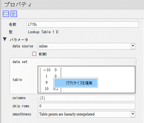
デフォルトのtableは[0 1 1]になっているので、その上あたりにマウスカーソルを持っていって右クリックすると図5のような「行列サイズを編集」というのが出てくるのでクリックします。
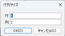
そうすると図6に示すような行列数をセットできるダイアログボックスが出てくるので、行列数を設定します。今回は4行2列にします。
1列目は入力に対応する数値で、2列目は出力に対応する数値を入力します。１列目の行は一番上が最も小さい数字を入れて、昇順に入力していきます。２列目は１列目のそれぞれの行の入力に対応する出力値です。

図5　「Lookup Table 1D」ブロックの設定（inlineの方法）

図 6　tableの行列数設定

【English】

This note introduces the use of interpolation calculations in MapleSim, which are commonly used in modeling. In particular, I will introduce a commonly used one-dimensional interpolation (Lookup Table 1D). Figure 1 shows a "Lookup Table 1D" block with a ramp input as an input for viewing the calculation results, and a gain block as a dummy behind the "Lookup Table 1D" block for probing the outputs.

Figure 1. "Lookup Table 1D" block

Create an interpolation table for the "Lookup Table 1D" block in a csv file. An example is shown in Figure 2.

Figure 2. csv file

Figure 3 shows the settings for the "Lookup Table 1D" block. The only things that need to be changed from the default settings are "data source" and "data. Set "data source" to "attachment. Next, select the csv file you created for "data."
That completes the setup. When you run the simulation, you will see the result as shown in Figure 4.

Figure 3. Setting up the "Lookup Table 1D" block

Figure 4. Calculation results

The "smoothness" is set to "Table points are linearly interpolated", so it is a linear interpolation. There are also spline interpolation and constant value interpolation. Also, as you can see in the result of Figure 4, extrapolation interpolation is performed. The way the extrapolation is calculated depends on the "smoothness" setting, but in the case of linear interpolation, it is an extension of the last two points. The positive side is an extension of the output values when the inputs are 9 and 10. The minus side is constant because they are the same values. Depending on how you want the extrapolated interpolation values to be, you need to clearly set the values in the csv file. If you do not want the extrapolation to be done without your permission, you need to explicitly enter the same values.

How to set up data in "inline"

There is also a way to directly input configuration values without creating a csv file. Set "data source" to "inline". The default is "inline". The default table is [0 1 1], so move the mouse cursor over the table and right-click, then click "Edit Matrix Size" as shown in Figure 5. A dialog box will then appear, as shown in Figure 6, in which you can set the number of matrices. The first row is the number corresponding to the input, the second row is the number corresponding to the output, and so on in ascending order. The second row is the output value corresponding to the input of each row in the first column.

Figure 5. Setting up the "Lookup Table 1D" block (inline)

Figure 6. Setting the number of matrices in table