
「ToyADMOS:異常音検知」:CNN

「ToyADMOS:異常音検知」手法比較:CNN と AutoEncoder の続きです。CNNのコードと実行結果サンプルを以下に示します。
概要
この例では、CNNをトレーニングします。
データセットは、ToyADAMOSのToyCar、Case4、CH1です。
このデータセットには、1335 の正常データ、263個の異常データが含まれ、それぞれに 528000 のデータポイントがあります。各例には、0(正常音)または1(異常音)のいずれかのラベルが付けられています。ここでは正常音、異常音の分類を目的としています。
CNNでは、波形をスペクトログラムに変換し、その2D画像をCNNで学習します。入力波形の正常・異常度合(確率)が出力され、確率の大きいラベルを採用します。
1.データセット:
ToyADAMOS:ToyCar, case4, CH1
2.コード(CNN)
モジュールのインポート
# 必要なモジュールと依存関係をインポート
import os
import pathlib

import matplotlib.pyplot as plt
import numpy as np
import seaborn as sns
import tensorflow as tf

from sklearn.metrics import classification_report
from tensorflow.keras import layers, losses
from tensorflow.keras import models
from IPython import display

# Set the seed value for experiment reproducibility.
seed = 42
tf.random.set_seed(seed)
np.random.seed(seed)
データセットやドライブの設定
# 対象の辞書
detect_targets_dict = {"car": 'ToyCar', "conv":'ToyConveyor', "train":'ToyTrain'}
detect_cases_dict = {"case1":'case1', "case2":'case2', "case3":'case3', "case4":'case4'}

# 対象を選択
detect_target = "car" # {"car": 'ToyCar', "conv":'ToyConveyor', "train":'ToyTrain'}
detect_case = "case4"
METHOD = 'CNN_'

# Googleドライブのマウント
from google.colab import drive
drive.mount('/content/drive')

#print("カレントワーキングディレクトリは[" + os.getcwd() + "]です")
_colab_dir = "/content/drive/MyDrive"
_colab_dir_program = _colab_dir+"/Anomaly_Detection/program"
_colab_dir_data = _colab_dir+"/Anomaly_Detection/data/"+detect_targets_dict[detect_target]+"/"+detect_cases_dict[detect_case]+"/ch1"
_folder_save = _colab_dir+"/Anomaly_Detection/result/CNN/"

os.chdir(_colab_dir_program)
print("カレントワーキングディレクトリは[" + os.getcwd() + "]です")
print("データディレクトリは[" + _colab_dir_data + "]です")
# サウンドデータセットをインポートするフォルダ
DATASET_PATH = _colab_dir_data
data_dir = pathlib.Path(DATASET_PATH)
データセットのオーディオクリップは、正常・異常コマンドに対応する2つのフォルダに保存されています:
# データセットのオーディオクリップは、
# 各サウンドに対応する2つのフォルダに保存されます:
#  'NormalSound_IND' 'AnormalousSound_IND'
commands = np.array(tf.io.gfile.listdir(str(data_dir)))
commands = sorted(commands, reverse=True)
print('Commands:', commands)
オーディオファイルの読込
オーディオクリップをfilenamesというリストに抽出し、シャッフルします。
# オーディオクリップをfilenamesというリストに抽出し、シャッフルします
filenames = tf.io.gfile.glob(str(data_dir) + '/*/*')
filenames = tf.random.shuffle(filenames)            # シャッフル
num_samples = len(filenames)
print('Number of total examples:', num_samples)
print('Number of NormalSound_IND per label:',
      len(tf.io.gfile.listdir(str(data_dir/commands[0]))))
print('Number of AnomalousSound_IND label:',
      len(tf.io.gfile.listdir(str(data_dir/commands[1]))))
print('Example file tensor:', filenames[0])
filenamesを、それぞれ80:10:10の比率を使用して、トレーニング、検証、およびテストセットに分割します。
# filenamesを、それぞれ80:10:10の比率を使用して、
# トレーニング、検証、およびテストセットに分割します。
train_counts = int(len(filenames) * 0.8)
val_counts = int(len(filenames) * 0.1)
test_counts = int(len(filenames) * 0.1)

train_files = filenames[:train_counts]
val_files = filenames[train_counts: train_counts + val_counts]
test_files = filenames[-1 * test_counts:]

print('Training set size', len(train_files))
print('Validation set size', len(val_files))
print('Test set size', len(test_files))
print('total_size', len(train_files) + len(val_files) + len(test_files))
オーディオファイルとそのラベルを設定
データセットを前処理し、波形と対応するラベルのデコードされたテンソルを作成します。
tf.audio.decode_wavによって返されるテンソルの形状は[samples, channels]です。ここで、 channelsはモノラルの場合は1 、ステレオの場合は2です。ミニ音声コマンドデータセットには、モノラル録音のみが含まれています。
# オーディオファイルの形状を確認
test_file = tf.io.read_file(filenames[0])  # file_pathを指定
test_audio, sampling_rate = tf.audio.decode_wav(contents=test_file)
# tf.audio.decode_wavによって返されるテンソルの形状は[samples, channels]
# channelsはモノラルの場合は1 、ステレオの場合は2
test_audio.shape
# Audio Setting
Data_num = test_audio.shape[0]
Sampling_freq = sampling_rate.numpy()
time_length = Data_num / Sampling_freq

print("Data数:", Data_num)
print("サンプリング周波数[Hz]:", Sampling_freq)
print("時間窓長[sec]:", time_length)
print("分析周波数レンジ[Hz]:", Sampling_freq / 2)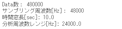
次に、データセットの生のWAVオーディオファイルをオーディオテンソルに前処理する関数を定義。
# データセットの生のWAVオーディオファイルをオーディオテンソルに前処理する関数を定義
# normalized to the [-1.0, 1.0] range
def decode_audio(audio_binary):
  audio, _ = tf.audio.decode_wav(contents=audio_binary)
  return tf.squeeze(audio, axis=-1) # モノラル信号のため、チャンネル軸を除去
各ファイルの親ディレクトリを使用してラベルを作成する関数を定義します。
# 各ファイルの親ディレクトリを使用してラベルを作成する関数
# ファイルパスをtf.RaggedTensorに分割します
def get_label(file_path):
  parts = tf.strings.split(
      input=file_path,
      sep=os.path.sep)
  return parts[-2]  # 最下層から2番目のフォルダ名を取得
すべてをまとめる別のヘルパー関数get_waveform_and_labelを定義します。
# すべてをまとめる別のヘルパー関数get_waveform_and_labelを定義
# 入力はWAVオーディオファイル名です。
# 出力は、教師あり学習の準備ができているオーディオテンソルとラベルテンソルを含むタプルです。
def get_waveform_and_label(file_path):
  label = get_label(file_path)
  audio_binary = tf.io.read_file(file_path)
  waveform = decode_audio(audio_binary)
  return waveform, label
音声とラベルのペアを抽出するためのトレーニングセットを作成します。後で同様の手順を使用して、検証セットとテストセットを作成します。
AUTOTUNE = tf.data.AUTOTUNE                                #

# 前に定義したget_waveform_and_labelを使用して、
# Dataset.from_tensor_slicesとDataset.mapを使用してtf.data.Datasetを作成します。

files_ds = tf.data.Dataset.from_tensor_slices(train_files) #

waveform_ds = files_ds.map(
    map_func=get_waveform_and_label,
    num_parallel_calls=AUTOTUNE) # トレーニングセット作成
いくつかのオーディオ波形をプロット。
# いくつかのオーディオ波形をプロット

rows = 3
cols = 3
n = rows * cols
fig, axes = plt.subplots(rows, cols, figsize=(10, 12))

for i, (audio, label) in enumerate(waveform_ds.take(n)):
  r = i // cols
  c = i % cols
  ax = axes[r][c]
  ax.plot(audio.numpy())
  ax.set_yticks(np.arange(-1.2, 1.2, 0.2))
  label = label.numpy().decode('utf-8')
  ax.set_title(label)

plt.show()

# ファイルを保存
fname = METHOD + detect_target + "_" + detect_case + '_wave.png'
path_save = _folder_save + fname
fig.savefig(path_save, dpi=64) #facecolor="lightgray", tight_layout=True)
波形をスペクトログラムに変換する
時間領域で表されたデータセット内の波形の短時間フーリエ変換(STFT)を計算して波形をスペクトログラムに変換します。
時間領域信号 ⇒ 時間周波数領域信号 ⇒ 2D画像(トレーニング)
STFT( tf.signal.stft )は、信号を時間のウィンドウに分割し、各ウィンドウでフーリエ変換を実行して、時間情報を保持し、標準の畳み込みを実行できる2Dテンソルを返します。
波形をスペクトログラムに変換するためのユーティリティ関数を作成します。
# 波形をスペクトログラムに変換
def get_spectrogram(waveform):
  # Cast the waveform tensors' dtype to float32.
  waveform = tf.cast(waveform, dtype=tf.float32)
  # Convert the waveform to a spectrogram via a STFT.
  spectrogram = tf.signal.stft(
      waveform, frame_length=255, frame_step=128) #
  # Obtain the magnitude of the STFT.
  spectrogram = tf.abs(spectrogram)
  spectrogram = spectrogram[..., tf.newaxis] # shape (`batch_size`, `height`, `width`, `channels`)
  return spectrogram
次に、データの調査を開始します。 1つの例のテンソル化された波形と対応するスペクトログラムの形状を印刷し、元のオーディオを再生します。
for waveform, label in waveform_ds.take(1):
  label = label.numpy().decode('utf-8')
  spectrogram = get_spectrogram(waveform)

print('Label:', label)
print('Waveform shape:', waveform.shape)
print('Spectrogram shape:', spectrogram.shape)
print('Audio playback')
display.display(display.Audio(waveform, rate=Sampling_Freq))
次に、スペクトログラムを表示するための関数を定義します。
# スペクトログラムを表示するための関数を定義
def plot_spectrogram(spectrogram, ax):
  if len(spectrogram.shape) > 2:
    assert len(spectrogram.shape) == 3
    spectrogram = np.squeeze(spectrogram, axis=-1)
  log_spec = np.log((spectrogram.T + np.finfo(float).eps) / np.finfo(float).eps) # Convert the frequencies to log scale and transpose
  height = log_spec.shape[0]
  width = log_spec.shape[1]
  X = np.linspace(0, np.size(spectrogram), num=width, dtype=int)
  Y = range(height)
  ax.pcolormesh(X, Y, log_spec)
時間の経過に伴う例の波形と対応するスペクトログラム(時間の経過に伴う周波数)をプロットします。
# 時間の経過に伴う例の波形と対応するスペクトログラム(時間の経過に伴う周波数)をプロット
fig, axes = plt.subplots(2, figsize=(12, 10))

axes[0].plot(waveform.numpy())
axes[0].set_title('Waveform')
axes[0].set_xlim([0, Data_num])
axes[0].grid()

plot_spectrogram(spectrogram.numpy(), axes[1])
axes[1].set_title('Spectrogram')

plt.show()

# ファイルを保存
fname = METHOD + detect_target + "_" + detect_case + '_wave_spect.png'
path_save = _folder_save + fname
fig.savefig(path_save, dpi=64) #facecolor="lightgray", tight_layout=True)
次に、波形データセットをスペクトログラムとそれに対応するラベルに整数IDとして変換する関数を定義します。
# 波形データセットをスペクトログラムとそれに対応するラベルに整数IDとして変換する関数を定義
def get_spectrogram_and_label_id(audio, label):
  spectrogram = get_spectrogram(audio)
  label_id = tf.argmax(label == commands)
  return spectrogram, label_id
get_spectrogram_and_label_idを使用して、データセットの要素全体にDataset.mapをマッピングします。
spectrogram_ds = waveform_ds.map(
  map_func=get_spectrogram_and_label_id,
  num_parallel_calls=AUTOTUNE)
データセットからいくつかの例についてスペクトログラムを確認します。
rows = 3
cols = 3
n = rows*cols
fig, axes = plt.subplots(rows, cols, figsize=(10, 10))

for i, (spectrogram, label_id) in enumerate(spectrogram_ds.take(n)):
  r = i // cols
  c = i % cols
  ax = axes[r][c]
  plot_spectrogram(spectrogram.numpy(), ax)
  ax.set_title(commands[label_id.numpy()])
  ax.axis('off')

plt.show()

# ファイルを保存
fname = METHOD + detect_target + "_" + detect_case + '_spectrogram.png'
path_save = _folder_save + fname
fig.savefig(path_save, dpi=64) #facecolor="lightgray", tight_layout=True)
モデルを構築してトレーニングする
検証セットとテストセットでトレーニングセットの前処理を繰り返します。
def preprocess_dataset(files):
  files_ds = tf.data.Dataset.from_tensor_slices(files)
  output_ds = files_ds.map(
      map_func=get_waveform_and_label,
      num_parallel_calls=AUTOTUNE)
  output_ds = output_ds.map(
      map_func=get_spectrogram_and_label_id,
      num_parallel_calls=AUTOTUNE)
  return output_ds
train_ds = spectrogram_ds # トレーニング用
val_ds = preprocess_dataset(val_files) # 検証用
test_ds = preprocess_dataset(test_files) # テスト用モデルトレーニングのトレーニングセットと検証セットをバッチ処理します。
batch_size = 64
train_ds = train_ds.batch(batch_size)
test_ds = test_ds.batch(batch_size)
set.cacheおよびDataset.prefetch操作を追加して、モデルのトレーニング中の読み取りレイテンシーを減らします。
train_ds = train_ds.cache().prefetch(AUTOTUNE)
test_ds = test_ds.cache().prefetch(AUTOTUNE)
val_ds = val_ds.cache().prefetch(AUTOTUNE)
モデルでは、オーディオファイルをスペクトログラム画像に変換したため、単純な畳み込みニューラルネットワーク(CNN)を使用します。
for spectrogram, _ in spectrogram_ds.take(1):
  input_shape = spectrogram.shape
print('Input shape:', input_shape)
num_labels = len(commands)

# Instantiate the `tf.keras.layers.Normalization` layer.
norm_layer = layers.Normalization()
# Fit the state of the layer to the spectrograms
# with `Normalization.adapt`.
norm_layer.adapt(data=spectrogram_ds.map(map_func=lambda spec, label: spec))

model = models.Sequential([
    layers.Input(shape=input_shape),
    # Downsample the input. 入力をダウンサンプリング
    layers.Resizing(32, 32),
    # Normalize. 平均と標準偏差に基づいて画像の各ピクセルを正規化
    norm_layer,
    layers.Conv2D(32, 3, activation='relu'),
    layers.Conv2D(64, 3, activation='relu'),
    layers.MaxPooling2D(), # 細かい位置情報削減しロバスト性を向上
    layers.Dropout(0.25),  # ランダムにニューロンを削除(0で上書き)
    layers.Flatten(),
    layers.Dense(128, activation='relu'),
    layers.Dropout(0.5),   # ランダムにニューロンを削除(0で上書き)
    layers.Dense(num_labels),
])

model.summary()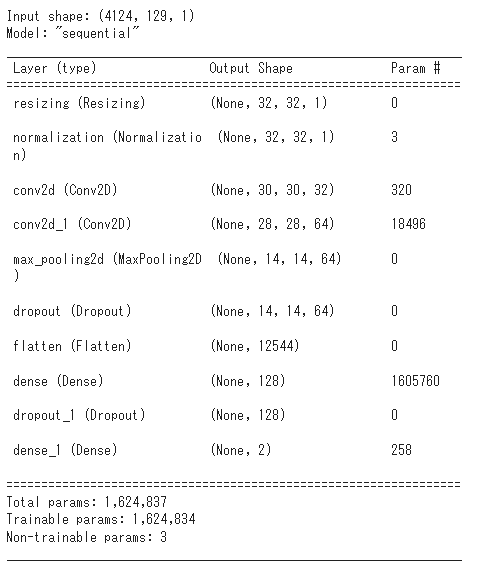
Adamオプティマイザーとクロスエントロピー損失を使用してKerasモデルを構成します。
Adamオプティマイザー:モーメンタム×RMSProp。
クロスエントロピー損失:分類の評価に特化 しているため、主に 分類モデルの誤差関数 として使われます。
# Adamオプティマイザーとクロスエントロピー損失を使用してKerasモデルを構成
model.compile(
optimizer=tf.keras.optimizers.Adam(),
loss=tf.keras.losses.SparseCategoricalCrossentropy(from_logits=True),
metrics=['accuracy'],
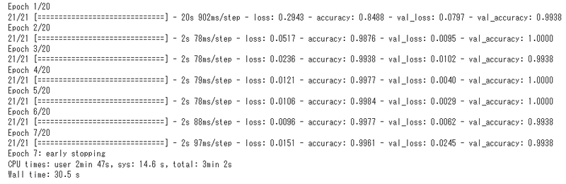
)モデルを20エポックまでトレーニングします。
EPOCHS = 20
history = model.fit(
    train_ds,
    validation_data=val_ds,
    epochs=EPOCHS,
    callbacks=tf.keras.callbacks.EarlyStopping(verbose=1, patience=2),
)
トレーニングと検証の損失曲線をプロットして、トレーニング中にモデルがどのように改善されたかを確認します。
metrics = history.history
fig = plt.figure(figsize=(16,6))
plt.subplot(1,2,1)
plt.plot(history.epoch, metrics['loss'], metrics['val_loss'])
plt.legend(['loss', 'val_loss'])
plt.ylim([0, max(plt.ylim())])
plt.xlabel('Epoch')
plt.ylabel('Loss [CrossEntropy]')
plt.title('Loss')

plt.subplot(1,2,2)
plt.plot(history.epoch, 100*np.array(metrics['accuracy']), 100*np.array(metrics['val_accuracy']))
plt.legend(['accuracy', 'val_accuracy'])
plt.ylim([0, 100])
plt.xlabel('Epoch')
plt.ylabel('Accuracy [%]')
plt.title('Accuracy')
# ファイルを保存
fname = METHOD + detect_target + "_" + detect_case + '_loss_accu.png'
path_save = _folder_save + fname
fig.savefig(path_save, dpi=64) #facecolor="lightgray", tight_layout=True)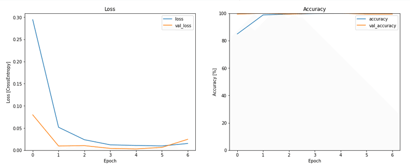
モデルのパフォーマンスを評価する
テストセットでモデルを実行し、モデルのパフォーマンスを確認します。
# testデータセットからaudioとラベルのデータセットを作成
test_audio = []
test_labels = []

for audio, label in test_ds:
  test_audio.append(audio.numpy())
  test_labels.append(label.numpy())

test_audio = np.array(test_audio)
test_labels = np.array(test_labels)
モデルのパフォーマンスを評価する
テストセットでモデルを実行し、モデルのパフォーマンスを確認します。
y_pred = np.argmax(model.predict(test_audio), axis=1)
y_true = test_labels
fname = METHOD + detect_target + "_" + detect_case + '_classification_report.csv'
path_save = _folder_save + fname
print(classification_report(y_true, y_pred,
target_names=commands))
report = classification_report(y_true, y_pred,
target_names=commands, output_dict=True) #
report_df = pd.DataFrame(report).T
report_df.to_csv(path_save)
混同行列を表示する
混合行列を使用して、モデルがテストセット内の各コマンドをどの程度適切に分類したかを確認します。
# 混同行列を表示する

confusion_mtx = tf.math.confusion_matrix(y_true, y_pred)
fig = plt.figure(figsize=(10, 8))
sns.heatmap(confusion_mtx,
            xticklabels=commands,
            yticklabels=commands,
            annot=True, fmt='g',annot_kws={"fontsize":17})
plt.xlabel('Prediction',fontsize=17)
plt.ylabel('Label',fontsize=17)
plt.show()

# ファイルを保存
fname = METHOD + detect_target + "_" + detect_case + '_confusion_mtx.png'
path_save = _folder_save + fname
fig.savefig(path_save, dpi=64) #facecolor="lightgray", tight_layout=True)
オーディオファイルで推論を実行する
最後に、「異常」の入力オーディオファイルを使用して、モデルの予測出力を確認します。99.9%の確率で異常と判定されました。
# オーディオファイルで推論を実行する
sample_file = filenames[4]
sample_ds = preprocess_dataset([sample_file])

fig = plt.figure(figsize=(10, 8))

for spectrogram, label in sample_ds.batch(1):
  prediction = model(spectrogram)
  plt.bar(commands, tf.nn.softmax(prediction[0]))
  plt.title(f'Predictions for "{commands[label[0]]}"')
  plt.show()

# ファイルを保存
fname = METHOD + detect_target + "_" + detect_case + '_predictions.png'
path_save = _folder_save + fname
fig.savefig(path_save, dpi=64) #facecolor="lightgray", tight_layout=True)

print(tf.nn.softmax(prediction[0]))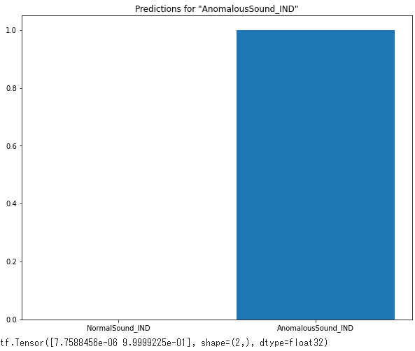
この記事が気に入ったらサポートをしてみませんか?