
Google Colabで時系列基盤モデルを試す④:amazon chronos-t5

はじめに
Google Timesfm、Moment、IBM Graniteに引き続き、HuggingFaceにある商用可能なライセンスの時系列基盤モデルを4つ試し、比較していきたいと思います。
利用するデータはETTh1という電力変圧器温度に関する多変量時系列データセットです。事前学習にこのデータが含まれる可能性があるため、モデルの絶対的な評価に繋がらないことに注意してください。
ダウンロード数:4.59k
モデルサイズ:200m
ライセンス:Apache-2.0
ダウンロード数:5.79k
モデルサイズ:385m
ライセンス:MIT
ibm-granite/granite-timeseries-ttm-v1
ダウンロード数:10.1k
モデルサイズ:805k (小さい!!)
ライセンス:Apache-2.0
ダウンロード数:256k (多い!!)
モデルサイズ:709m
ライセンス:Apache-2.0
6月2日時点でダウンロード数が少ない順に実施していきます。
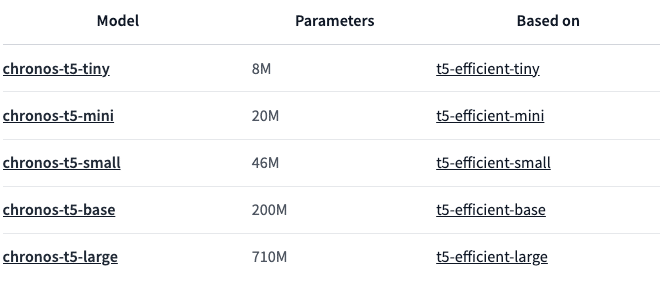
今回はamazonのchronos-t5です。このモデルはMomentと同様にT5をベースにしているようです。また、このモデルは5種類のサイズを提供しています。
特に、largeは他のモデルと比べても最も大きいサイズです。性能に期待ができます。
1. 推論
ライブラリの準備
# library install
!pip install git+https://github.com/amazon-science/chronos-forecasting.git
データ準備
これまで同様ETTh1.csvを使います。取得はこちらから可能です。
import pandas as pd

# データ読み込み
# https://github.com/zhouhaoyi/ETDataset/blob/main/ETT-small/ETTh1.csv
df = pd.read_csv("ETTh1.csv")
print(len(df))
df.head(2)
データは以下のような形式です。OT(Oil Temperature)が目的変数となります。

データ加工
モデルに与える長さを512、予測する長さを96と今回はおきます。Fine Tuningに使うため、後ろから予測するデータをとっておきます。
Timesfmと同じ形式のTensorを使います。
import torch

context_length = 512
forecast_horizon = 96

# データセット分割
df_train = df.iloc[-(context_length+forecast_horizon):-forecast_horizon]
df_test = df.iloc[-forecast_horizon:]

# 形式の変更
train_tensor = torch.tensor(df_train[["HUFL", "HULL", "MUFL", "MULL", "LUFL", "LULL", "OT"]].values, dtype=torch.float)
train_tensor = train_tensor.t()
test_tensor = torch.tensor(df_test[["HUFL", "HULL", "MUFL", "MULL", "LUFL", "LULL", "OT"]].values, dtype=torch.float)
test_tensor = test_tensor.t()
モデルPipelineの定義
モデルでの推論をより手軽に行えるPipelineが提供されていたためこちらを使います。基本的な使い方はTransformersのpipelineと同様です。
import pandas as pd
import torch
from chronos import ChronosPipeline

pipeline = ChronosPipeline.from_pretrained(
    "amazon/chronos-t5-large",
    device_map="cuda",  # use "cpu" for CPU inference and "mps" for Apple Silicon
    torch_dtype=torch.bfloat16,
)
pipelineを表示してみると、modelは以下のような構成です。MeanScaleUniformBinsというTokenizerとT5のChronosModelを使用しています。
ChronosPipeline(tokenizer=<chronos.chronos.MeanScaleUniformBins object at 0x7e656c3bf250>, model=ChronosModel(
  (model): T5ForConditionalGeneration(
    (shared): Embedding(4096, 1024)
    (encoder): T5Stack(
      (embed_tokens): Embedding(4096, 1024)
      (block): ModuleList(
        (0): T5Block(
          (layer): ModuleList(
            (0): T5LayerSelfAttention(
              (SelfAttention): T5Attention(
                (q): Linear(in_features=1024, out_features=1024, bias=False)
                (k): Linear(in_features=1024, out_features=1024, bias=False)
                (v): Linear(in_features=1024, out_features=1024, bias=False)
                (o): Linear(in_features=1024, out_features=1024, bias=False)
                (relative_attention_bias): Embedding(32, 16)
              )
              (layer_norm): T5LayerNorm()
              (dropout): Dropout(p=0.1, inplace=False)
            )
            (1): T5LayerFF(
              (DenseReluDense): T5DenseActDense(
                (wi): Linear(in_features=1024, out_features=4096, bias=False)
                (wo): Linear(in_features=4096, out_features=1024, bias=False)
                (dropout): Dropout(p=0.1, inplace=False)
                (act): ReLU()
              )
              (layer_norm): T5LayerNorm()
              (dropout): Dropout(p=0.1, inplace=False)
            )
          )
        )
        (1-23): 23 x T5Block(
          (layer): ModuleList(
            (0): T5LayerSelfAttention(
              (SelfAttention): T5Attention(
                (q): Linear(in_features=1024, out_features=1024, bias=False)
                (k): Linear(in_features=1024, out_features=1024, bias=False)
                (v): Linear(in_features=1024, out_features=1024, bias=False)
                (o): Linear(in_features=1024, out_features=1024, bias=False)
              )
              (layer_norm): T5LayerNorm()
              (dropout): Dropout(p=0.1, inplace=False)
            )
            (1): T5LayerFF(
              (DenseReluDense): T5DenseActDense(
                (wi): Linear(in_features=1024, out_features=4096, bias=False)
                (wo): Linear(in_features=4096, out_features=1024, bias=False)
                (dropout): Dropout(p=0.1, inplace=False)
                (act): ReLU()
              )
              (layer_norm): T5LayerNorm()
              (dropout): Dropout(p=0.1, inplace=False)
            )
          )
        )
      )
      (final_layer_norm): T5LayerNorm()
      (dropout): Dropout(p=0.1, inplace=False)
    )
    (decoder): T5Stack(
      (embed_tokens): Embedding(4096, 1024)
      (block): ModuleList(
        (0): T5Block(
          (layer): ModuleList(
            (0): T5LayerSelfAttention(
              (SelfAttention): T5Attention(
                (q): Linear(in_features=1024, out_features=1024, bias=False)
                (k): Linear(in_features=1024, out_features=1024, bias=False)
                (v): Linear(in_features=1024, out_features=1024, bias=False)
                (o): Linear(in_features=1024, out_features=1024, bias=False)
                (relative_attention_bias): Embedding(32, 16)
              )
              (layer_norm): T5LayerNorm()
              (dropout): Dropout(p=0.1, inplace=False)
            )
            (1): T5LayerCrossAttention(
              (EncDecAttention): T5Attention(
                (q): Linear(in_features=1024, out_features=1024, bias=False)
                (k): Linear(in_features=1024, out_features=1024, bias=False)
                (v): Linear(in_features=1024, out_features=1024, bias=False)
                (o): Linear(in_features=1024, out_features=1024, bias=False)
              )
              (layer_norm): T5LayerNorm()
              (dropout): Dropout(p=0.1, inplace=False)
            )
            (2): T5LayerFF(
              (DenseReluDense): T5DenseActDense(
                (wi): Linear(in_features=1024, out_features=4096, bias=False)
                (wo): Linear(in_features=4096, out_features=1024, bias=False)
                (dropout): Dropout(p=0.1, inplace=False)
                (act): ReLU()
              )
              (layer_norm): T5LayerNorm()
              (dropout): Dropout(p=0.1, inplace=False)
            )
          )
        )
        (1-23): 23 x T5Block(
          (layer): ModuleList(
            (0): T5LayerSelfAttention(
              (SelfAttention): T5Attention(
                (q): Linear(in_features=1024, out_features=1024, bias=False)
                (k): Linear(in_features=1024, out_features=1024, bias=False)
                (v): Linear(in_features=1024, out_features=1024, bias=False)
                (o): Linear(in_features=1024, out_features=1024, bias=False)
              )
              (layer_norm): T5LayerNorm()
              (dropout): Dropout(p=0.1, inplace=False)
            )
            (1): T5LayerCrossAttention(
              (EncDecAttention): T5Attention(
                (q): Linear(in_features=1024, out_features=1024, bias=False)
                (k): Linear(in_features=1024, out_features=1024, bias=False)
                (v): Linear(in_features=1024, out_features=1024, bias=False)
                (o): Linear(in_features=1024, out_features=1024, bias=False)
              )
              (layer_norm): T5LayerNorm()
              (dropout): Dropout(p=0.1, inplace=False)
            )
            (2): T5LayerFF(
              (DenseReluDense): T5DenseActDense(
                (wi): Linear(in_features=1024, out_features=4096, bias=False)
                (wo): Linear(in_features=4096, out_features=1024, bias=False)
                (dropout): Dropout(p=0.1, inplace=False)
                (act): ReLU()
              )
              (layer_norm): T5LayerNorm()
              (dropout): Dropout(p=0.1, inplace=False)
            )
          )
        )
      )
      (final_layer_norm): T5LayerNorm()
      (dropout): Dropout(p=0.1, inplace=False)
    )
    (lm_head): Linear(in_features=1024, out_features=4096, bias=False)
  )
))
推論
以下のコードで推論が可能です。これまでのモデルとは違い、chronosはポイント予測ではなく確率予測をします。つまり、1時間単位に対して(デフォルトでは)20の予測される値を出力します。従って、グラフに線として出力する際にはmean、もしくはmedianを取る必要があります。
予測長(forecast_horizon)としては64以下が推奨されるようで、これまで通りに96を指定すると注意されます。そこで、limit_prediction_length=Falseと指定することで96まで予測することができるようになります。
# 推論
forecast = pipeline.predict(train_tensor, forecast_horizon, limit_prediction_length=False)
forecast_median_tensor, _ = torch.median(forecast, dim=1)
Google ColabのT4を使い、推論には30秒ほどかかりました。
また、(他モデルでは気にしてませんでしたが)使用メモリは10GBほどで自宅用のPCでの頻繁な利用は厳しいなと感じました。(LLMよりは全然軽量ですが。)

推論結果の出力
予測結果としてOT(Oil Temperature)がみたいのでchannel_idxとして6を指定します。
import matplotlib.pyplot as plt

channel_idx = 6
time_index = 0

history = train_tensor[channel_idx, :].detach().numpy()
true = test_tensor[channel_idx, :].detach().numpy()
pred = forecast_median_tensor[channel_idx, :].detach().numpy()

plt.figure(figsize=(12, 4))

# Plotting the first time series from history
plt.plot(range(len(history)), history, label='History (512 timesteps)', c='darkblue')

# Plotting ground truth and prediction
num_forecasts = len(true)

offset = len(history)
plt.plot(range(offset, offset + len(true)), true, label='Ground Truth (96 timesteps)', color='darkblue', linestyle='--', alpha=0.5)
plt.plot(range(offset, offset + len(pred)), pred, label='Forecast (96 timesteps)', color='red', linestyle='--')

plt.title(f"ETTh1 (Hourly) -- (idx={time_index}, channel={channel_idx})", fontsize=18)
plt.xlabel('Time', fontsize=14)
plt.ylabel('Value', fontsize=14)
plt.legend(fontsize=14)
plt.show()
結果は以下のようになります。
モデルサイズが大きいだけあり、これまでのモデルと比べて最も精度良く予測できている気がします。推奨されている予測長64以降もきちんと予測できています。
(予測がはまりすぎていて、事前学習にETTh1が含まれているのではと思いました。)

2. Fine Tuning
Google ColabのT4ではメモリが足りなかったため、A100に切り替えました。
ライブラリ準備
コードが長くなりそうだったので、提供されているのTrain用スクリプトを使っていきます。
!pip install "chronos[training] @ git+https://github.com/amazon-science/chronos-forecasting.git"
!git clone https://github.com/amazon-science/chronos-forecasting.git
データ準備
Trainスクリプトに投げる用のデータファイルを出力します。
import pandas as pd

context_length = 512
forecast_horizon = 96

# ETTh1.csvを読み込む
df = pd.read_csv("ETTh1.csv")

# データを前8割をトレーニング用、後ろ2割をテスト用に分割
train_size = int(0.8 * len(df))
print(train_size)
df_train = df.iloc[:train_size]
df_test = df.iloc[train_size:-(context_length+forecast_horizon)]
from pathlib import Path
from typing import List, Optional, Union
import numpy as np
from gluonts.dataset.arrow import ArrowWriter
def convert_to_arrow(
path: Union[str, Path],
time_series: Union[List[np.ndarray], np.ndarray],
start_times: Optional[Union[List[np.datetime64], np.ndarray]] = None,
compression: str = "lz4",
):
if start_times is None:
# Set an arbitrary start time
start_times = [np.datetime64("2000-01-01 00:00", "s")] * len(time_series)
assert len(time_series) == len(start_times)
dataset = [
{"start": start, "target": ts} for ts, start in zip(time_series, start_times)
]
ArrowWriter(compression=compression).write_to_file(
dataset,
path=path,
)
# Convert to GluonTS arrow format
cols = ["HUFL", "HULL", "MUFL", "MULL", "LUFL", "LULL", "OT"]
convert_to_arrow(
path = "./etth1-train.arrow",
time_series=[np.array(df_train[col]) for col in cols],
start_times=[pd.to_datetime(df_train["date"]).values[0]] * len(cols),
)モデル準備
# Load model
model = TinyTimeMixerForPrediction.from_pretrained(
    "ibm/TTM", revision=TTM_MODEL_REVISION, head_dropout=0.7
)

# Freeze the backbone of the model
for param in model.backbone.parameters():
    param.requires_grad = False
諸々の設定
他モデルと同様に1epochだけ学習させます。Trainスクリプトにmax_epochsを指定できなかったため、1epochとなるようにnum_stepsを計算します。
また、本来はbatch_sizeも他モデルと揃えて64としたかったのですがA100でもメモリが足りず、8としました。
import yaml

batch_size = 8
num_steps = train_size/batch_size

# 書き出したいデータを辞書形式で定義
config_data = {
    'training_data_paths': [
        "./etth1-train.arrow",
    ],
    'probability': [1.0],
    'output_dir': './output/',
    'context_length': 512,
    'prediction_length': 96,
    'max_steps': num_steps,
    'per_device_train_batch_size': batch_size,
    'learning_rate': 0.001,
    'model_id': 'amazon/chronos-t5-large',
    'random_init': False,
    'tf32': True,  # turn False this if not using Ampere GPUs (e.g., A100)
}

# yamlファイルに書き出すパス
config_path = '/content/ft_config.yaml'

# 辞書データをyamlファイルに書き出す
with open(config_path, 'w') as file:
    yaml.dump(config_data, file)Optimizer等の宣言
Trainスクリプトの実行
先に書き出しておいたconfigファイルを渡します。GPUは1つなので頭にCUDA_VISIBLE_DEVICES=0とつけます。マルチGPUの場合は下に記載してあるようにtorchrun --nproc-per-node=8とするようです。
実行には18分かかりました。GPUメモリは31GBほどだったと思います。
# Fine Tuningの実行
!CUDA_VISIBLE_DEVICES=0 python chronos-forecasting/scripts/training/train.py --config /content/ft_config.yaml

# On multiple GPUs (example with 8 GPUs)
# torchrun --nproc-per-node=8 training/train.py --config /path/to/modified/config.yaml
モデル保存
最後にFineTuningしたモデルをHuggingFaceにプッシュしました。プッシュしたモデルはこちらになります。
from chronos import ChronosPipeline

pipeline = ChronosPipeline.from_pretrained("./output/run-1/checkpoint-final/")
pipeline.model.model.push_to_hub("chronos-t5-large-ft-etth1-1ep")
3. 推論(Fine Tuning後)
最後に、先に試したのと同じ区間で推論を再度実施してみます。
データ準備
import torch

context_length = 512
forecast_horizon = 96

# データセット分割
df_train = df.iloc[-(context_length+forecast_horizon):-forecast_horizon]
df_test = df.iloc[-forecast_horizon:]

# 形式の変更
train_tensor = torch.tensor(df_train[["HUFL", "HULL", "MUFL", "MULL", "LUFL", "LULL", "OT"]].values, dtype=torch.float)
train_tensor = train_tensor.t()
test_tensor = torch.tensor(df_test[["HUFL", "HULL", "MUFL", "MULL", "LUFL", "LULL", "OT"]].values, dtype=torch.float)
test_tensor = test_tensor.t()
モデルの取得
プッシュしたモデルを取得します。
import pandas as pd
import torch
from chronos import ChronosPipeline

pipeline = ChronosPipeline.from_pretrained(
    "HachiML/chronos-t5-large-ft-etth1-1ep",
    device_map="cuda",  # use "cpu" for CPU inference and "mps" for Apple Silicon
    torch_dtype=torch.bfloat16,
)
推論
# 推論
forecast = pipeline.predict(train_tensor, forecast_horizon, limit_prediction_length=False)
forecast_median_tensor, _ = torch.median(forecast, dim=1)
推論結果の出力
import matplotlib.pyplot as plt

channel_idx = 6
time_index = 0

history = train_tensor[channel_idx, :].detach().numpy()
true = test_tensor[channel_idx, :].detach().numpy()
pred = forecast_median_tensor[channel_idx, :].detach().numpy()

plt.figure(figsize=(12, 4))

# Plotting the first time series from history
plt.plot(range(len(history)), history, label='History (512 timesteps)', c='darkblue')

# Plotting ground truth and prediction
num_forecasts = len(true)

offset = len(history)
plt.plot(range(offset, offset + len(true)), true, label='Ground Truth (96 timesteps)', color='darkblue', linestyle='--', alpha=0.5)
plt.plot(range(offset, offset + len(pred)), pred, label='Forecast (96 timesteps)', color='red', linestyle='--')

plt.title(f"ETTh1 (Hourly) -- (idx={time_index}, channel={channel_idx})", fontsize=18)
plt.xlabel('Time', fontsize=14)
plt.ylabel('Value', fontsize=14)
plt.legend(fontsize=14)
plt.show()
結果は以下のようになりました。2山目以降のフィット感が若干増したような気がしますが、元々かなり予測できていたので0-shotで十分という感じもしました。

4. 結果
これまでで最もサイズの大きいモデルであり、これまでで最も精度良く予測できている気がします。また、FineTuningも問題なく実行できました。
一方で、推論やFine Tuningにメモリを結構使ったので、前回のgraniteとchronosで場面によって使い分けたりすることになるかもなと考えさせられました。(まだ時系列の基盤モデルは使い所が定まっていないと思うのでその辺りもこれから考えられていくのだろうなと思います。)
また、他モデルと異なり確率予測だったのが特徴的でした。
今回はポイント予測のモデルと比較していたのでしなかったですが、以下のように信頼区間のようなものもグラフ表示することができます。

import matplotlib.pyplot as plt
import numpy as np

channel_idx = 6
time_index = 0

history = train_tensor[channel_idx, :].detach().numpy()
true = test_tensor[channel_idx, :].detach().numpy()
pred = forecast_median_tensor[channel_idx, :].detach().numpy()
low, median, high = np.quantile(forecast[channel_idx].numpy(), [0.1, 0.5, 0.9], axis=0)

plt.figure(figsize=(12, 4))

# Plotting the first time series from history
plt.plot(range(len(history)), history, label='History (512 timesteps)', c='darkblue')

# Plotting ground truth and prediction
num_forecasts = len(true)

offset = len(history)
plt.plot(range(offset, offset + len(true)), true, label='Ground Truth (96 timesteps)', color='darkblue', linestyle='--', alpha=0.5)
plt.plot(range(offset, offset + len(pred)), pred, label='Forecast (96 timesteps)', color='red', linestyle='--')
plt.fill_between(range(offset, offset + len(pred)), low, high, color="tomato", alpha=0.3, label="80% prediction interval")

plt.title(f"ETTh1 (Hourly) -- (idx={time_index}, channel={channel_idx})", fontsize=18)
plt.xlabel('Time', fontsize=14)
plt.ylabel('Value', fontsize=14)
plt.legend(fontsize=14)
plt.show()
参照
この記事が気に入ったらサポートをしてみませんか?