OceanParcels(2) ~Quickstart to Parcels(2)

引き続きOceanParcelsのQuickstart to Parcelsのページを訳しながら進める

Quickstart to Parcels — Parcels v3.0.0-19-g67d3931 documentation

Running particles in backward time

お次は逆輸送を考えるらしい。なんか簡単とか言ってる
dt < 0を考えてやるらしい

まずは同様に、必要なモジュール類をimportする

import math
from datetime import timedelta
from operator import attrgetter

import matplotlib.pyplot as plt
import numpy as np
import trajan as ta
import xarray as xr
from IPython.display import HTML
from matplotlib.animation import FuncAnimation

from parcels import (
    AdvectionRK4,
    FieldSet,
    JITParticle,
    ParticleSet,
    Variable,
    download_example_dataset,
)

particlesetまでの流れは同じ（前回参照）

example_dataset_folder = download_example_dataset("MovingEddies_data")
fieldset = FieldSet.from_parcels(f"{example_dataset_folder}/moving_eddies")

fieldset.computeTimeChunk(time=0, dt=1)

##particleset

pset = ParticleSet.from_list(
    fieldset=fieldset,  # particleを投入するfieldの指定
    pclass=JITParticle,  # 粒子の種類 (JITParticle と ScipyParticleの2種類がある)
    lon=[3.3e5, 3.3e5],  
    lat=[1e5, 2.8e5],  
)

##field　と particle の図示

##＃field の図示
#plt.pcolormesh(fieldset.U.grid.lon, fieldset.U.grid.lat, fieldset.U.data[0, :, :])
#plt.xlabel("Zonal distance [m]")
#plt.ylabel("Meridional distance [m]")
#plt.colorbar()

### particle の図示
#plt.plot(pset.lon, pset.lat, "ko") # 粒子を黒い丸い点で示す
#plt.show()

##karnelset

###出力先のファイルを指定する
output_file = pset.ParticleFile(
    name="EddyParticles_Bwd.zarr",  # ファイルの名前
    outputdt=timedelta(hours=1),  # 出力のtime stepを指定
)

###実際に計算する
pset.execute(
    AdvectionRK4,  # 使用するkarnelを指定
    runtime=timedelta(days=6),  # runの長さを指定
    dt=-timedelta(minutes=5),  # kernelのtimestepを指定、ここでマイナスにすることで逆輸送できる
    output_file=output_file,
)

重要なのは最後のブロック4行目の
dt=-timedelta(minutes=5)
においてtimedeltaの前にマイナス記号がついていることだ、これにより逆向きの推定ができるようになる

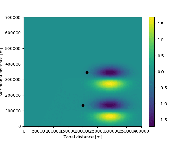
図の表示は同様

plt.pcolormesh(fieldset.U.grid.lon, fieldset.U.grid.lat, fieldset.U.data[0, :, :])
plt.xlabel("Zonal distance [m]")
plt.ylabel("Meridional distance [m]")
plt.colorbar()

plt.plot(pset.lon, pset.lat, "ko")
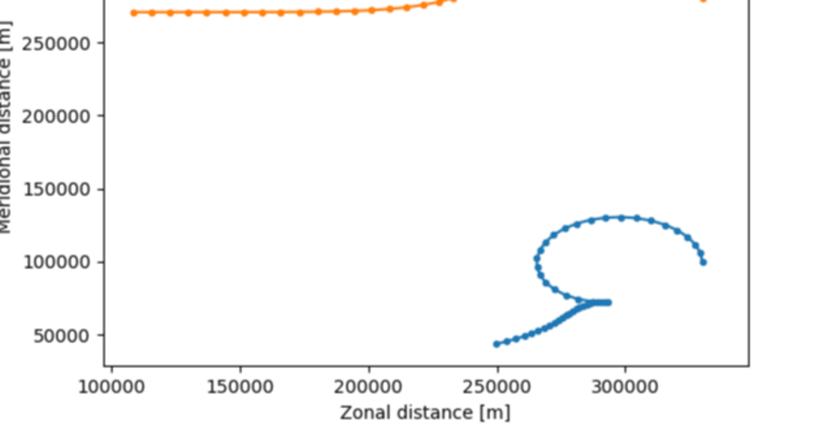
plt.show()

OceanParticlesのページはすでに6日の設定で走らせたものを巻き戻しているが、そうではなく初期位置から6日間巻き戻す設定で走らせてみると以下のような図が得られる

Adding a custom behaviour kernel

a simple kernel where particles obtain an extra 2 m/s westward velocity after 1 day
つまり粒子は1日後にさらに2m/sの西向きの速度を得るようなkernelを作成する

def Westvel(particle, fieldset, time):
    if time > 86400: #1日後になったら
    uvel = -2.0, #追加する流速の設定
    particle_dlon += uvel * particle.dt 

The Parcels Kernel loop — Parcels v3.0.0-19-g67d3931 documentation

ここのparticle_dlonがどういうものなのか…
とりあえずここは私も理解しないまま、後で勉強する…ということにする。
↓

上記コマンドをparticlesetに入れ込んで、再度partclesetを実行する。
そして以下のコマンドを実行する。pset.execute()内のKarnelを指定するところが、[AdvectionRK4, WestVel]となっていてWestVelが入っていることに注意。意外に簡単に加えることができる。

### particle の投入

pset = ParticleSet.from_list(
    fieldset=fieldset,  # particleを投入するfieldの指定
    pclass=JITParticle,  # 粒子の種類 (JITParticle と ScipyParticleの2種類がある)
    lon=[3.3e5, 3.3e5],  
    lat=[1e5, 2.8e5],  
)

##karnelset

###出力先のファイルを指定する
output_file = pset.ParticleFile(
    name="EddyParticles_WestVel.zarr",  # ファイルの名前
    outputdt=timedelta(hours=1),  # 出力のtime stepを指定
)

###実際に計算する

pset.execute(
    [AdvectionRK4, WestVel],  # 使用するkarnelを指定、単純にカーネルをリストにまとめる
    runtime=timedelta(days=2),
    dt=timedelta(minutes=5),
    output_file=output_file,
)

なお、前回の逆輸送のコードを改変して再利用する場合、
dt = -timedelta(minutes=5)
の-を必ず外すこと、外さないと処理が途中で止まってしまう。
またoutputのファイル名は変える

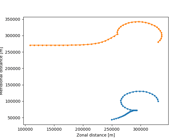
そして以下のコードで図に出力

ds = xr.open_zarr("EddyParticles_WestVel.zarr")

plt.xlabel("Zonal distance [m]")
plt.ylabel("Meridional distance [m]")
plt.plot(pset.lon, pset.lat, ".-")
plt.show()

以下が出力結果