OceanParcels日記 ~Quickstart to Parcels(1)

2023年11月12日 01:40

OceanParcelsのQuickstart to Parcelsのページを訳しながら進める

以下はOceanParcelsのページの目次

Running particles in an idealised field

まずは必要なモジュール類をimportする

import math
from datetime import timedelta
from operator import attrgetter

import matplotlib.pyplot as plt
import numpy as np
import trajan as ta
import xarray as xr
from IPython.display import HTML
from matplotlib.animation import FuncAnimation

from parcels import (
    AdvectionRK4,
    FieldSet,
    JITParticle,
    ParticleSet,
    Variable,
    download_example_dataset,
)

trajanは軌跡を扱うpythonのpackage

まずは2つの理想化された動く渦の単純な流れを考えるらしい。

fieldset

そのためのfieldsetを以下でダウンロード

example_dataset_folder = download_example_dataset("MovingEddies_data")

fieldset = FieldSet.from_parcels(f"{example_dataset_folder}/moving_eddies")

このfieldsetを可視化したい。そのためにmatplotlib.pyplot.pcolormesh関数を使うとのこと。
https://matplotlib.org/stable/api/_as_gen/matplotlib.pyplot.pcolormesh.html
MatplotlibとはMatplotlibは、プログラミング言語Pythonおよびその科学計算用ライブラリNumPyのためのグラフ描画ライブラリ（Wikipedia）のことらしい。

まずはZonal Velocity: U(球の赤道に平行なパターンに従う流束)を可視化する

#fieldsetの最初の時間フレームを読み込む
fieldset.computeTimeChunk(time=0, dt=1)

plt.pcolormesh(fieldset.U.grid.lon, fieldset.U.grid.lat, fieldset.U.data[0, :, :])
plt.xlabel("Zonal distance [m]")
plt.ylabel("Meridional distance [m]")
plt.colorbar()
plt.show()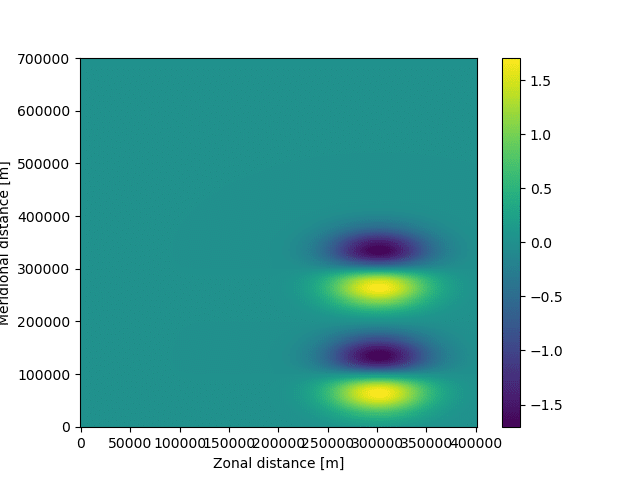

これでfieldsetの準備は完了。

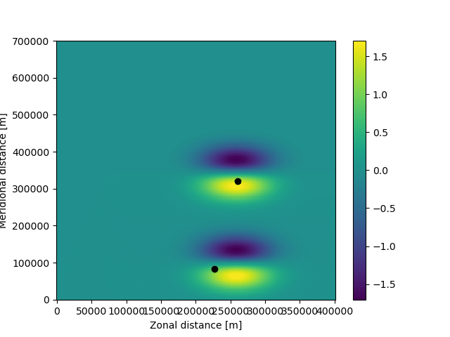
particleset

次にparticlesetを準備する。(lon, lat)が(330km, 100km)と(330km, 280km)の2点に粒子を投入するのが以下のコード。

pset = ParticleSet.from_list(
    fieldset=fieldset,  # particleを投入するfieldの指定
    pclass=JITParticle,  # 粒子の種類 (JITParticle と ScipyParticleの2種類がある)
    lon=[3.3e5, 3.3e5],  
    lat=[1e5, 2.8e5],  
)

print (pset)
#結果
#P[0](lon=330000.000000, lat=100000.000000, depth=0.000000, time=not_yet_set)
#P[1](lon=330000.000000, lat=280000.000000, depth=0.000000, time=not_yet_set)

fieldsetで扱った図の可視化のコードに
plt.plot(pset.lon, pset.lat, "ko")
というコードを加えてあげれば、粒子の位置を入れ込むことができるそうな
ちなみにkoはマーカーの色や形の指定。詳しくは以下のサイトを参照

上記のページより以下の画像を引用
今回はk、つまり黒色で、加えてo、つまり丸型のマーカーを指定している

話は戻るが、可視化のコードは以下のようになる
下記のコードは粒子の位置やラベルなどを、先ほど出力した図に重ね合わせる

plt.pcolormesh(fieldset.U.grid.lon, fieldset.U.grid.lat, fieldset.U.data[0, :, :])
plt.xlabel("Zonal distance [m]")
plt.ylabel("Meridional distance [m]")
plt.colorbar()

plt.plot(pset.lon, pset.lat, "ko") #粒子を図内に表示することを指示している
plt.show()

ここまでを一気に実行すると、以下の図が得られる

ここまででfieldとparticleのセットが終わったので、最後にkarnelのセットに入る。

karnelset

今回はRunge-Kutta法を用いたkarnelで走らせてみるらしい。
Runge-Kutta法とは"初期値問題に対して近似解を与える常微分方程式の数値解法に対する総称"らしい
参考）

5分ごとの計算で6日分走らせる。軌跡情報は1時間ごとのものをEddyParticles.zarrというファイルに格納する。
参考）zarr形式

以下のコードを書く

#出力先のファイルを指定する
output_file = pset.ParticleFile(
    name="EddyParticles.zarr",  # ファイルの名前
    outputdt=timedelta(hours=1),  # 出力のtime stepを指定
)

#実際に計算する
pset.execute(
    AdvectionRK4,  # 使用するkarnelを指定
    runtime=timedelta(days=6),  # runの長さを指定
    dt=timedelta(minutes=5),  # kernelのtimestepを指定
    output_file=output_file,
)

これで走らせると以下の図が出てくる
これは6日間、走り終わった後の粒子の位置を示す
流速の分布も、粒子の位置も変わっていることがわかる

xr.open_zarr()という関数を使ってあげれば、zaaファイルを開いて軌道を示してあげることができる

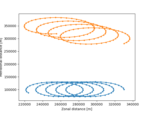
ds = xr.open_zarr("EddyParticles.zarr") #ファイルを開いて、変数に保存

plt.plot(ds.lon.T, ds.lat.T, ".-") #.-"はプロットの点や線の形の指定
plt.xlabel("Zonal distance [m]")
plt.ylabel("Meridional distance [m]")
plt.show()

ここでds.lon.Tや、ds.lat.Tのように転置されているのはds.lonが (time, y, x) のような形でzarrに格納されているからである。
plt.plot は(x, y, time) の形で読み込みたいため、ds.lon.Tのように転置して (x, y, time) にしてから読み込ませる

上記のコードを実行すると以下のような図が得られる

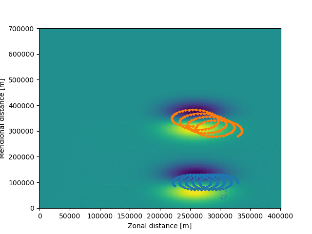
なお上記のコードに

plt.pcolormesh(fieldset.U.grid.lon, fieldset.U.grid.lat, fieldset.U.data[0, :, :])

を足してから図示すると以下のようになる

アニメーション化

ただこれだけに飽き足らず、FuncAnimation()関数を使ってあげると、軌跡をアニメーションで表示できるようである

%%capture #セルの結果を出力するマジックコマンド、プロットされた図が表示されるのを防ぐため
fig = plt.figure(figsize=(7, 5), constrained_layout=True) #図の様式の指定
ax = fig.add_subplot() #図に加えるアニメーションを格納するaxを作成

ax.set_ylabel("Meridional distance [m]")
ax.set_xlabel("Zonal distance [m]")
ax.set_xlim(0, 4e5)
ax.set_ylim(0, 7e5)

# アニメーションの出力を早めるため、5つごとのtimestepで考える
timerange = np.unique(ds["time"].values)[::5]

# 最初の時間に対応するデータのインデックスを取得
time_id = np.where(ds["time"] == timerange[0]) 

# 散布図を作成し、初期時点での粒子の位置をプロットする
sc = ax.scatter(ds["lon"].values[time_id], ds["lat"].values[time_id]) 

# タイトルの設定（図の中央上部に表示されるやつ）
t = str(timerange[0].astype("timedelta64[h]")) #最初の時間に対応する文字列を作成、astype("timedelta[]")で時間の単位を指定
title = ax.set_title(f"Particles at t = {t}") 


def animate(i):
    t = str(timerange[i].astype("timedelta64[h]"))
    title.set_text(f"Particles at t = {t}")

    time_id = np.where(ds["time"] == timerange[i])
    sc.set_offsets(np.c_[ds["lon"].values[time_id], ds["lat"].values[time_id]])


anim = FuncAnimation(fig, animate, frames=len(timerange), interval=100)
#Matplotlibのアニメーションクラスで、animate関数を使用してアニメーションを作成。framesはアニメーションの総フレーム数、intervalは各フレームの表示時間を指定
anim.save('animation.gif', writer='imagemagick')

以上を実行すると以下のようなアニメーションファイルが生成され、current directory内に保存される
クリックすると表示される、なんかカクカクするのはなんでだろう…実際はカクカクしてない

まとめ

import math
from datetime import timedelta
from operator import attrgetter

import matplotlib.pyplot as plt
import numpy as np
import trajan as ta
import xarray as xr
from IPython.display import HTML
from matplotlib.animation import FuncAnimation

from parcels import (
    AdvectionRK4,
    FieldSet,
    JITParticle,
    ParticleSet,
    Variable,
    download_example_dataset,
)


#Running particles in an idealised field

##fieldset

example_dataset_folder = download_example_dataset("MovingEddies_data")
fieldset = FieldSet.from_parcels(f"{example_dataset_folder}/moving_eddies")

fieldset.computeTimeChunk(time=0, dt=1)

##particleset

pset = ParticleSet.from_list(
    fieldset=fieldset,  # particleを投入するfieldの指定
    pclass=JITParticle,  # 粒子の種類 (JITParticle と ScipyParticleの2種類がある)
    lon=[3.3e5, 3.3e5],  
    lat=[1e5, 2.8e5],  
)

##field　と particle の図示

##＃field の図示
#plt.pcolormesh(fieldset.U.grid.lon, fieldset.U.grid.lat, fieldset.U.data[0, :, :])
#plt.xlabel("Zonal distance [m]")
#plt.ylabel("Meridional distance [m]")
#plt.colorbar()

### particle の図示
#plt.plot(pset.lon, pset.lat, "ko") # 粒子を黒い丸い点で示す
#plt.show()

##karnelset

###出力先のファイルを指定する
output_file = pset.ParticleFile(
    name="EddyParticles.zarr",  # ファイルの名前
    outputdt=timedelta(hours=1),  # 出力のtime stepを指定
)

###実際に計算する
pset.execute(
    AdvectionRK4,  # 使用するkarnelを指定
    runtime=timedelta(days=6),  # runの長さを指定
    dt=timedelta(minutes=5),  # kernelのtimestepを指定
    output_file=output_file,
)

### 軌道の図示

ds = xr.open_zarr("EddyParticles.zarr") #ファイルを開いて、変数に保存

#plt.plot(ds.lon.T, ds.lat.T, ".-") #.-"はプロットの点や線の形の指定
#plt.xlabel("Zonal distance [m]")
#plt.ylabel("Meridional distance [m]")
#plt.show()

#%%capture #セルの結果を出力するマジックコマンド、プロットされた図が表示されるのを防ぐため
fig = plt.figure(figsize=(7, 5), constrained_layout=True) #図の様式の指定
ax = fig.add_subplot() #図に加えるアニメーションを格納するaxを作成

ax.set_ylabel("Meridional distance [m]")
ax.set_xlabel("Zonal distance [m]")
ax.set_xlim(0, 4e5)
ax.set_ylim(0, 7e5)

# アニメーションの出力を早めるため、5つごとのtimestepで考える
timerange = np.unique(ds["time"].values)[::5]

# 最初の時間に対応するデータのインデックスを取得
time_id = np.where(ds["time"] == timerange[0]) 

# 散布図を作成し、初期時点での粒子の位置をプロットする
sc = ax.scatter(ds["lon"].values[time_id], ds["lat"].values[time_id]) 

# タイトルの設定（図の中央上部に表示されるやつ）
t = str(timerange[0].astype("timedelta64[h]")) #最初の時間に対応する文字列を作成、astype("timedelta[]")で時間の単位を指定
title = ax.set_title(f"Particles at t = {t}") 


def animate(i):
    t = str(timerange[i].astype("timedelta64[h]"))
    title.set_text(f"Particles at t = {t}")

    time_id = np.where(ds["time"] == timerange[i])
    sc.set_offsets(np.c_[ds["lon"].values[time_id], ds["lat"].values[time_id]])


anim = FuncAnimation(fig, animate, frames=len(timerange), interval=100)
#Matplotlibのアニメーションクラスで、animate関数を使用してアニメーションを作成。framesはアニメーションの総フレーム数、intervalは各フレームの表示時間を指定
anim.save('animation.gif', writer='imagemagick')

この記事が気に入ったらサポートをしてみませんか？