
機械学習(回帰)⑴〜データ取込・前処理〜

BRIXIT Journal note第2弾ということで、今回は社長酒巻の弟であり、
データサイエンティストをしている裕也がお送りします。
よろしくお願いします。
今回は私が最初に勉強がてら使っていたKaggleのチュートリアルであるHouse Price (住宅販売価格予測)を簡単な実例と共にご紹介致します。
大まかな流れをご紹介するので、数式等は記述しませんのでご了承下さい。
因みに、Pythonのバージョンは3.6.3を使用しています。
機械学習の基本的な流れ
データ取込 :DBやCSV・EXCELファイルなど
前処理 :特徴量として使える形に加工
学習・予測 :データによりモデルを選定
精度検証 :回帰→RMSE, 分類→accuracy等で精度確認
今回行ったKaggleのチュートリアルでは予測対象の正解データがないので、
Kaggleで表示されるScoreを基に検証をしていきます。
【データ取込】
■基本的なライブラリのインポート
import pandas as pd
import numpy as np
# データ可視化
import matplotlib.pyplot as plt
%matplotlib inline
import seaborn as sns
■データ読み込み
Kaggleに会員登録し、House Priceのページに行くとデータセットをダウンロードできます。ディレクトリ構成は単一ディレクトリのみで行います。
train_df = pd.read_csv('train.csv')
test_df = pd.read_csv('test.csv')
【前処理】
■データ量と基本統計量の確認
train_df.shape
(1460, 81)
test_df.shape
(1459, 80)
train_dfには1460行、81列のデータが確認できました。
では実際にどのようなデータがあるのか見ていきます。
# リストだと長いのでarrayで表示
np.array(train_df.columns)

array(['Id', 'MSSubClass', 'MSZoning', 'LotFrontage', 'LotArea', 'Street',
      'Alley', 'LotShape', 'LandContour', 'Utilities', 'LotConfig',
      'LandSlope', 'Neighborhood', 'Condition1', 'Condition2', 'BldgType',
      'HouseStyle', 'OverallQual', 'OverallCond', 'YearBuilt',
      'YearRemodAdd', 'RoofStyle', 'RoofMatl', 'Exterior1st',
      'Exterior2nd', 'MasVnrType', 'MasVnrArea', 'ExterQual', 'ExterCond',
      'Foundation', 'BsmtQual', 'BsmtCond', 'BsmtExposure',
      'BsmtFinType1', 'BsmtFinSF1', 'BsmtFinType2', 'BsmtFinSF2',
      'BsmtUnfSF', 'TotalBsmtSF', 'Heating', 'HeatingQC', 'CentralAir',
      'Electrical', '1stFlrSF', '2ndFlrSF', 'LowQualFinSF', 'GrLivArea',
      'BsmtFullBath', 'BsmtHalfBath', 'FullBath', 'HalfBath',
      'BedroomAbvGr', 'KitchenAbvGr', 'KitchenQual', 'TotRmsAbvGrd',
      'Functional', 'Fireplaces', 'FireplaceQu', 'GarageType',
      'GarageYrBlt', 'GarageFinish', 'GarageCars', 'GarageArea',
      'GarageQual', 'GarageCond', 'PavedDrive', 'WoodDeckSF',
      'OpenPorchSF', 'EnclosedPorch', '3SsnPorch', 'ScreenPorch',
      'PoolArea', 'PoolQC', 'Fence', 'MiscFeature', 'MiscVal', 'MoSold',
      'YrSold', 'SaleType', 'SaleCondition', 'SalePrice'], dtype=object)
敷地面積や屋根の形状、車庫の有無など様々な条件があることが
分かりました。
予測対象の目的変数は最後の「SalePrice」にあたります。
次にSalePriceの基本統計量を見ていきます。
Pythonではdescribe()を使うことで簡単に確認できます。
train_df['SalePrice'].describe()

count      1460.000000
mean     180921.195890
std       79442.502883
min       34900.000000
25%      129975.000000
50%      163000.000000
75%      214000.000000
max      755000.000000
Name: SalePrice, dtype: float64
最大値と最小値に大きな差がありますね。
グラフでも確認してみましょう。
plt.style.use('ggplot')
fig = plt.figure()
ax = fig.add_subplot(1,1,1)
ax.hist(train_df['SalePrice'], bins=50)
ax.set_ylim(0,200)
fig.show()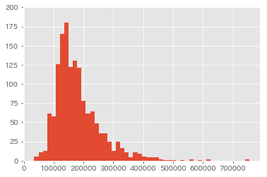
可視化することで、データに偏りが確認できました。
このままでは外れ値が大きく影響してしまう為、
データを正規化していきます。
train_id = train_df['Id']
test_id = test_df['Id']
y_train = train_df['SalePrice']
x_train = train_df.drop(['Id'], axis=1)
x_test = test_df.drop(['Id'], axis=1)
X_all = pd.concat((x_train, x_test))
y_train = np.log(y_train)
sns.distplot(y_train)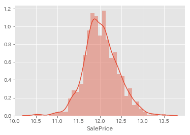
■データ欠損値の処理
実務でも多々ありますが、データの欠損値処理って言っちゃ悪いが
結構面倒くさい作業です。(笑)
データとしての「0」と「無し」では意味が大きく変わってしまうので、
この欠損値処理をどうするかによって精度にも影響してくる大事な作業です。
欠損値を確認していきましょう。
# 欠損値の個数を確認
X_all.isnull().sum()[X_all.isnull().sum()!=0].sort_values(ascending=False)

PoolQC          2909
MiscFeature     2814
Alley           2721
Fence           2348
SalePrice       1459
FireplaceQu     1420
LotFrontage      486
GarageQual       159
GarageCond       159
GarageFinish     159
GarageYrBlt      159
GarageType       157
BsmtExposure      82
BsmtCond          82
BsmtQual          81
BsmtFinType2      80
BsmtFinType1      79
MasVnrType        24
MasVnrArea        23
MSZoning           4
BsmtFullBath       2
BsmtHalfBath       2
Utilities          2
Functional         2
Electrical         1
BsmtUnfSF          1
Exterior1st        1
Exterior2nd        1
TotalBsmtSF        1
GarageCars         1
BsmtFinSF2         1
BsmtFinSF1         1
KitchenQual        1
SaleType           1
GarageArea         1
dtype: int64
# heatmapで欠損箇所を確認
sns.heatmap(train_df.isnull(), cbar=False)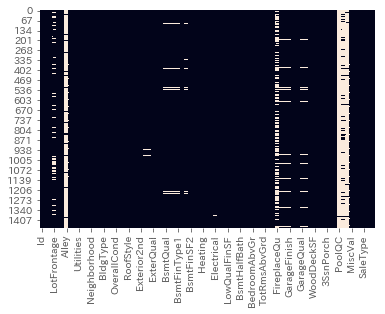
データの欠損はSalePrice合わせて35項目となりました。多い……
では補完していきます。今回は4種類に分けて補完していきます。
### 欠損値の補完
# 0で補完
X_all['LotFrontage'].fillna(0, inplace=True)
X_all['GarageYrBlt'].fillna(0, inplace=True)
X_all['MasVnrArea'].fillna(0, inplace=True)
X_all['BsmtFullBath'].fillna(0, inplace=True)
X_all['BsmtHalfBath'].fillna(0, inplace=True)
X_all['BsmtFinSF1'].fillna(0, inplace=True)
X_all['BsmtFinSF2'].fillna(0, inplace=True)
X_all['BsmtUnfSF'].fillna(0, inplace=True)
X_all['GarageCars'].fillna(0, inplace=True)
X_all['GarageArea'].fillna(0, inplace=True)
X_all['TotalBsmtSF'].fillna(0, inplace=True)
# NAという文字列で補完
X_all['PoolQC'].fillna('NA', inplace=True)
X_all['Alley'].fillna('NA', inplace=True)
X_all['Fence'].fillna('NA', inplace=True)
X_all['FireplaceQu'].fillna('NA', inplace=True)
X_all['GarageFinish'].fillna('NA', inplace=True)
X_all['GarageQual'].fillna('NA', inplace=True)
X_all['GarageCond'].fillna('NA', inplace=True)
X_all['GarageType'].fillna('NA', inplace=True)
X_all['BsmtExposure'].fillna('NA', inplace=True)
X_all['BsmtCond'].fillna('NA', inplace=True)
X_all['BsmtQual'].fillna('NA', inplace=True)
X_all['BsmtFinType2'].fillna('NA', inplace=True)
X_all['BsmtFinType1'].fillna('NA', inplace=True)
X_all['MasVnrType'].fillna('NA', inplace=True)
# Noneという文字列で補完
X_all['MiscFeature'].fillna('None', inplace=True)
# 最頻値で補完
X_all['MSZoning'] = X_all['MSZoning'].fillna(X_all['MSZoning'].mode()[0])
X_all['Utilities'] = X_all['Utilities'].fillna(X_all['Utilities'].mode()[0])
X_all['Functional'] = X_all['Functional'].fillna(X_all['Functional'].mode()[0])
X_all['Exterior2nd'] = X_all['Exterior2nd'].fillna(X_all['Exterior2nd'].mode()[0])
X_all['Exterior1st'] = X_all['Exterior1st'].fillna(X_all['Exterior1st'].mode()[0])
X_all['SaleType'] = X_all['SaleType'].fillna(X_all['SaleType'].mode()[0])
X_all['Electrical'] = X_all['Electrical'].fillna(X_all['Electrical'].mode()[0])
X_all['KitchenQual'] = X_all['KitchenQual'].fillna(X_all['KitchenQual'].mode()[0])
ちゃんと補完できたか再度可視化して確認。

SalePrice以外が補完できました。
■特徴量の加工
文字列データはそのままでは特徴量として使うことができない為、
数値化しないといけません。
まず確認データ型を確認します。
X_all.dtypes

1stFlrSF           int64
2ndFlrSF           int64
3SsnPorch          int64
Alley             object
BedroomAbvGr       int64
BldgType          object
BsmtCond          object
BsmtExposure      object
BsmtFinSF1       float64
BsmtFinSF2       float64
BsmtFinType1      object
BsmtFinType2      object
BsmtFullBath     float64
BsmtHalfBath     float64
BsmtQual          object
BsmtUnfSF        float64
CentralAir        object
Condition1        object
Condition2        object
Electrical        object
EnclosedPorch      int64
ExterCond         object
ExterQual         object
Exterior1st       object
Exterior2nd       object
Fence             object
FireplaceQu       object
Fireplaces         int64
Foundation        object
FullBath           int64
                 ...
LotShape          object
LowQualFinSF       int64
MSSubClass         int64
MSZoning          object
MasVnrArea       float64
MasVnrType        object
MiscFeature       object
MiscVal            int64
MoSold             int64
Neighborhood      object
OpenPorchSF        int64
OverallCond        int64
OverallQual        int64
PavedDrive        object
PoolArea           int64
PoolQC            object
RoofMatl          object
RoofStyle         object
SaleCondition     object
SalePrice        float64
SaleType          object
ScreenPorch        int64
Street            object
TotRmsAbvGrd       int64
TotalBsmtSF      float64
Utilities         object
WoodDeckSF         int64
YearBuilt          int64
YearRemodAdd       int64
YrSold             int64
Length: 80, dtype: object
dtypeを入力すると、各カラムのデータ型が確認できます。
objectと書いてある箇所が今回変換したい項目です。
Pythonでは便利なライブラリ、その名も「ラベルエンコーダー」なるものがあります。
早速使ってみましょう。
# ラベルエンコーダーでSTRを数値化
from sklearn.preprocessing import LabelEncoder

for i in range(X_all.shape[1]):
   # columnsがobjectのものだけ変換する
   if X_all.iloc[:,i].dtypes == object:
       lbl = LabelEncoder()
       lbl.fit(list(X_all.iloc[:,i].values))
       X_all.iloc[:,i] = lbl.transform(list(X_all.iloc[:,i].values))
ちゃんと変換出来たか確認↓
X_all.dtypes

1stFlrSF           int64
2ndFlrSF           int64
3SsnPorch          int64
Alley              int64
BedroomAbvGr       int64
BldgType           int64
BsmtCond           int64
BsmtExposure       int64
BsmtFinSF1       float64
BsmtFinSF2       float64
BsmtFinType1       int64
BsmtFinType2       int64
BsmtFullBath     float64
BsmtHalfBath     float64
BsmtQual           int64
BsmtUnfSF        float64
CentralAir         int64
Condition1         int64
Condition2         int64
Electrical         int64
EnclosedPorch      int64
ExterCond          int64
ExterQual          int64
Exterior1st        int64
Exterior2nd        int64
Fence              int64
FireplaceQu        int64
Fireplaces         int64
Foundation         int64
FullBath           int64
                 ...
LotShape           int64
LowQualFinSF       int64
MSSubClass         int64
MSZoning           int64
MasVnrArea       float64
MasVnrType         int64
MiscFeature        int64
MiscVal            int64
MoSold             int64
Neighborhood       int64
OpenPorchSF        int64
OverallCond        int64
OverallQual        int64
PavedDrive         int64
PoolArea           int64
PoolQC             int64
RoofMatl           int64
RoofStyle          int64
SaleCondition      int64
SalePrice        float64
SaleType           int64
ScreenPorch        int64
Street             int64
TotRmsAbvGrd       int64
TotalBsmtSF      float64
Utilities          int64
WoodDeckSF         int64
YearBuilt          int64
YearRemodAdd       int64
YrSold             int64
Length: 80, dtype: object
PoolQL等を見てみると、objectからint64になりました。
これで特徴量として使えるようになりました。
ここからtrain, test用に再度データを分割します。
n_train = train_df.shape[0]
train = X_all[:n_train]
x_test = X_all[n_train:]
y = y_train
X = train.drop(['SalePrice'],axis=1)
ライブラリの中にはRandomForestやLightGBMのように、
どの特徴量がモデルとして重要度が高いのか確認することも出来ます。
# ランダムフォレストで特徴量を調べる
from sklearn.ensemble import RandomForestRegressor
rf = RandomForestRegressor(n_estimators=20, max_features='auto')
rf.fit(X, y)

ranking = np.argsort(-rf.feature_importances_)
f, ax = plt.subplots(figsize=(11,9))
sns.barplot(x=rf.feature_importances_[ranking],
           y=X.columns.values[ranking],
           orient='h')
ax.set_xlabel("feature importance")
plt.tight_layout()
plt.show()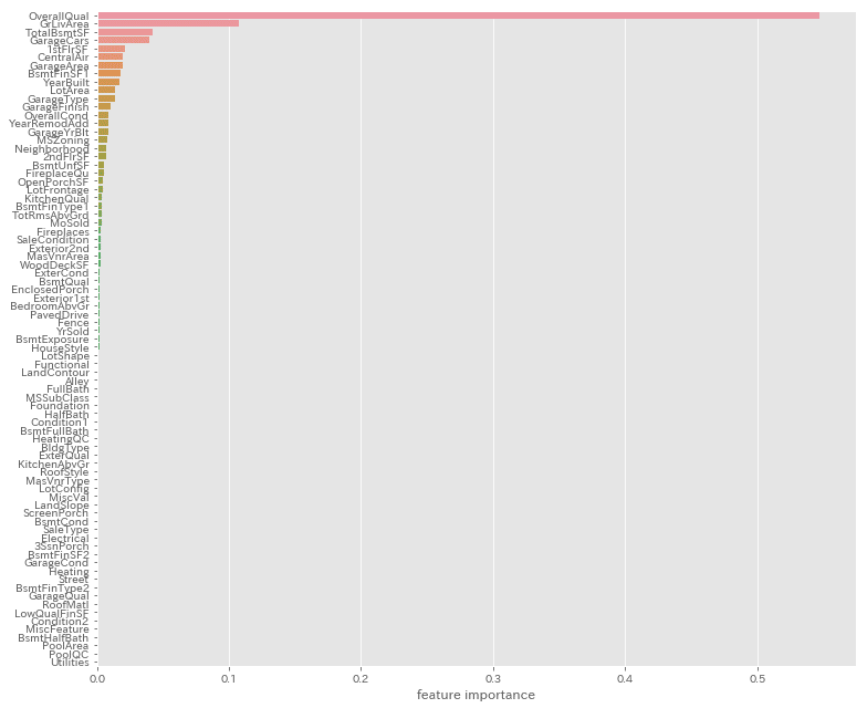
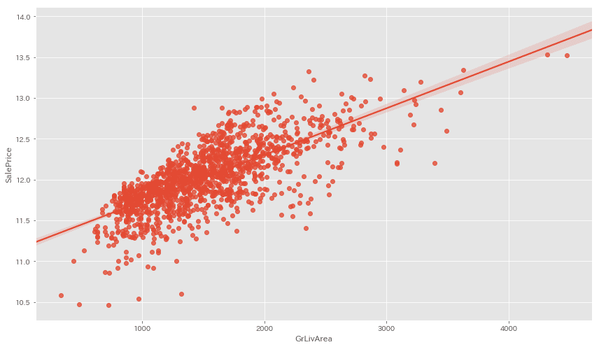
■外れ値の確認
データには凡そ平均から大きく離れた外れ値というものがあります。
重要度の高いTOP3を見てみましょう。
cols_list = ['OverallQual', 'TotalBsmtSF', 'GrLivArea']
for cols in cols_list:
   fig = plt.figure(figsize=(12,7))
   sns.regplot(x=X[cols], y=y)
   plt.tight_layout()
   plt.show()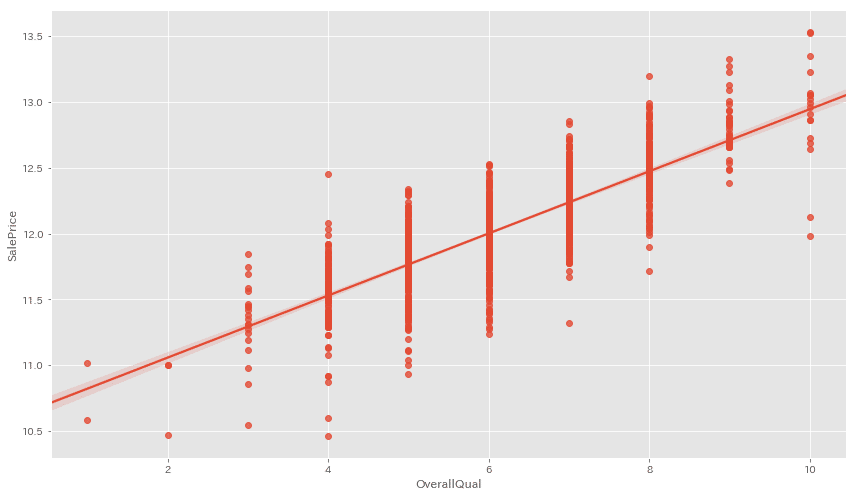
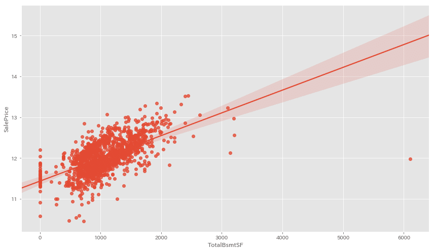
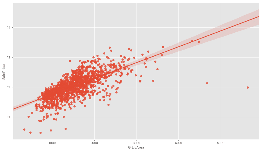
OverallQualは特別外れ値がある訳ではなさそう。。。
TotalBsmtSFとGrLivAreaには近似線から大きく外れた値が見られますね。
今回はこちらの外れ値を除いて前処理を終えたいと思います。
# 外れ値を取り除く
X_mat = X
X_mat = pd.concat([X_mat,y], axis=1)
X_mat = X_mat.drop(X_mat[(X_mat['TotalBsmtSF'] > 6000)].index)
X_mat = X_mat.drop(X_mat[(X_mat['GrLivArea']>4600)].index)

X_train = X_mat.drop(['SalePrice'], axis=1)
y_train = X_mat['SalePrice']
取り除けたか再可視化して確認します。
cols_list = ['TotalBsmtSF', 'GrLivArea']
for cols in cols_list:
   fig = plt.figure(figsize=(12,7))
   sns.regplot(x=X_train[cols], y=y_train)
   plt.tight_layout()
   plt.show()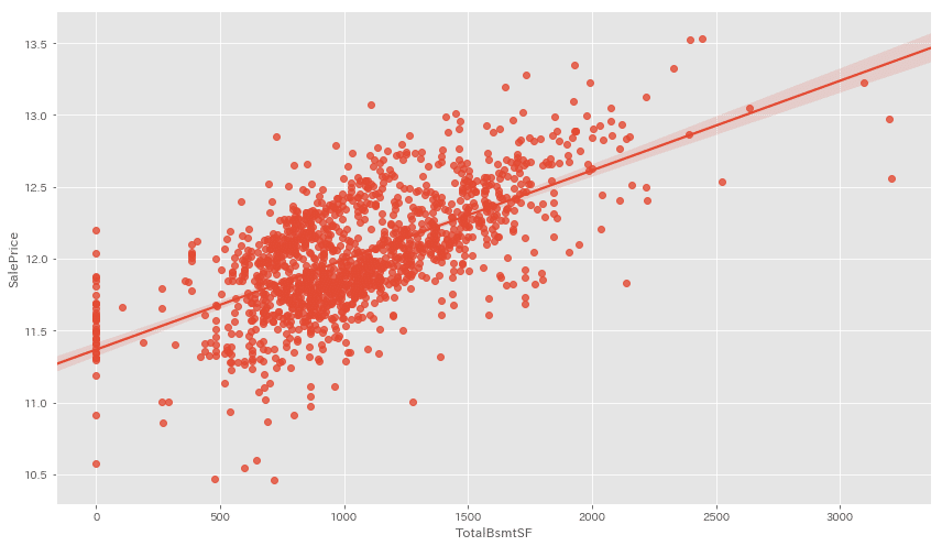
外れ値がしっかり無くなっていることが確認出来ました!
実務ではこの数十倍くらいの分析〜前処理をしますが、
今回は分析も程々に簡単な前処理を行ってきました。
次回(2)では、作成したデータを使って実際に機械学習モデルへ
適用していきたいと思います!
この記事が気に入ったらサポートをしてみませんか?