Theo Jansen機構をお絵描きしてみよう

この記事は,機械系Advent Calendar 2020の23日の記事として書いています.付け焼刃の記事ではありますが,最後まで読んでいただけると幸いです.最後のGIFアニメだけでも見ていってください…!
要約
機構学の授業で登場した,Theo Jansen機構のお絵描きをPythonを使ってしました.ソースコードはこちら↓にあります.ぜひいじってみてください.(編集権限がない旨のエラーでると思います.「ファイル」→「コピーを保存」をしてから再度試してみてください.)
Theo Jansen機構とは
Theo Jansen機構とは,オランダの彫刻家Theo Jansen(1948-)の作品ストランドビーストに用いられているリンク機構です.直線的な機械要素のみで構成されているにもかかわらず,非常に生物的な動きをします.YouTubeにも動画が上がっています.
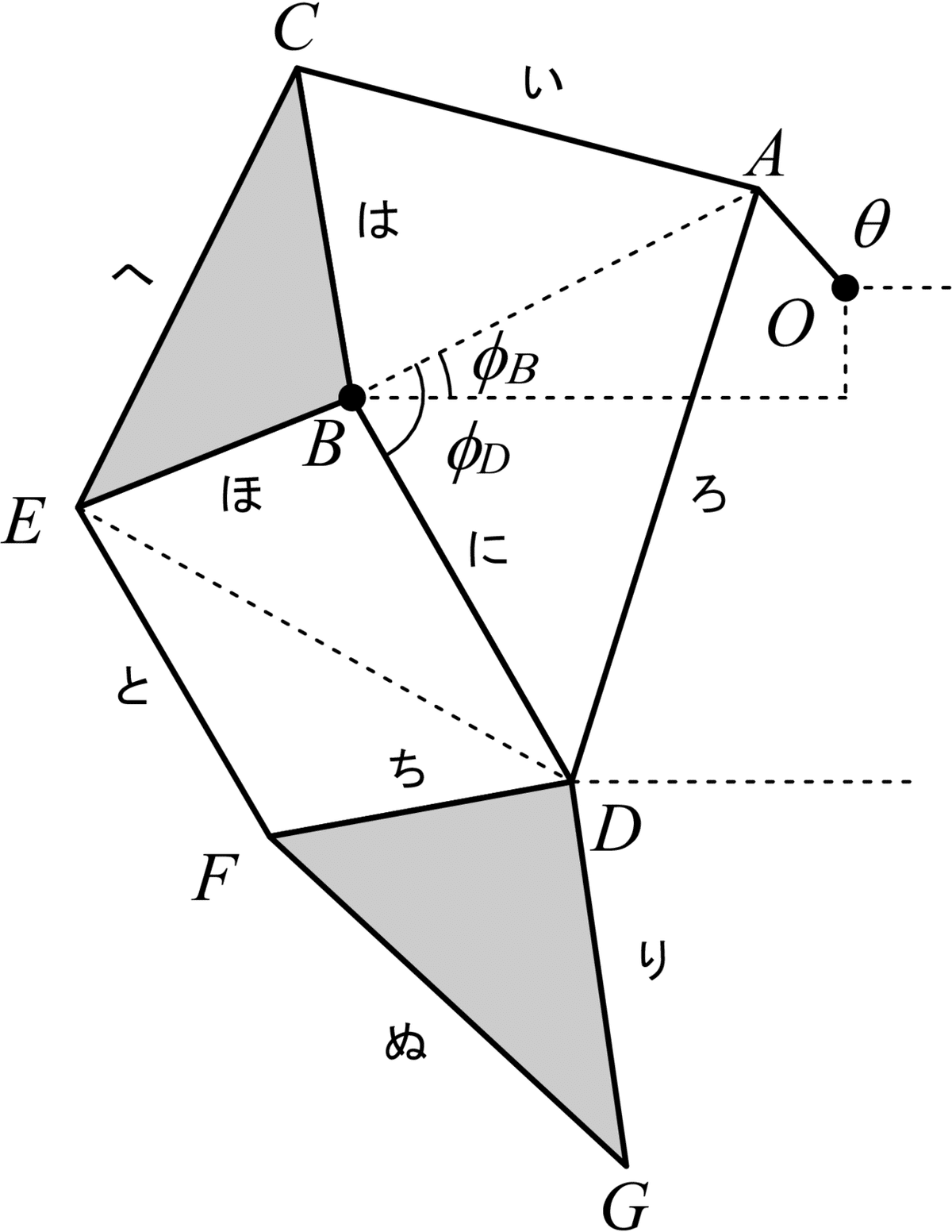
リンクおよび対偶の定義
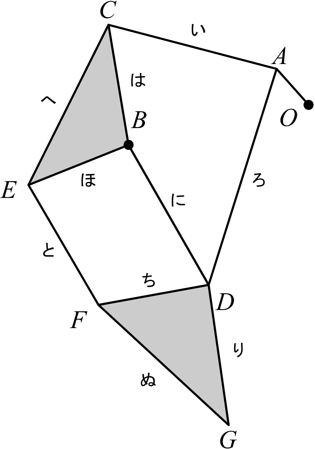
次の様にリンクおよび節の名前を定義します.アルファベットが点対偶で,平仮名がリンクです.
リンク機構は,リンクOAを回転させることで機構全体が動きます.そこで,回転を簡単に扱うことのできる複素数平面で考えていきます.それぞれの点の位置をZA,ZB,...と表すことととします.
点Oおよび点Bは固定点で,点Aは角速度ωで回転するため,
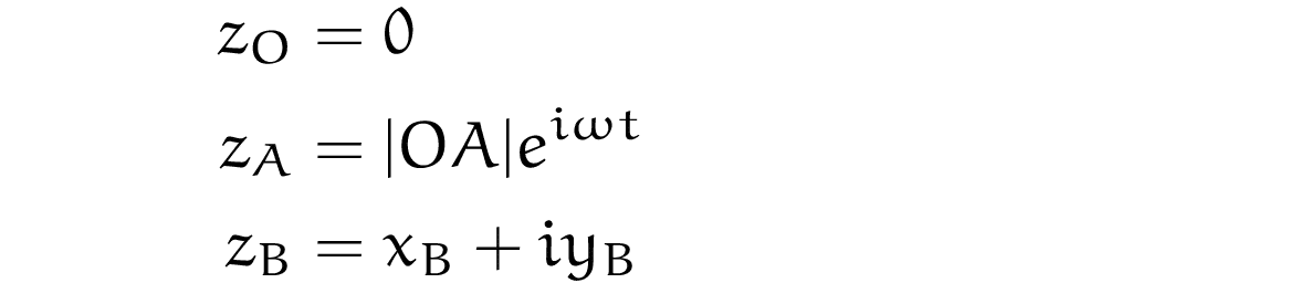
となります.
点C,点Eの位置を求める
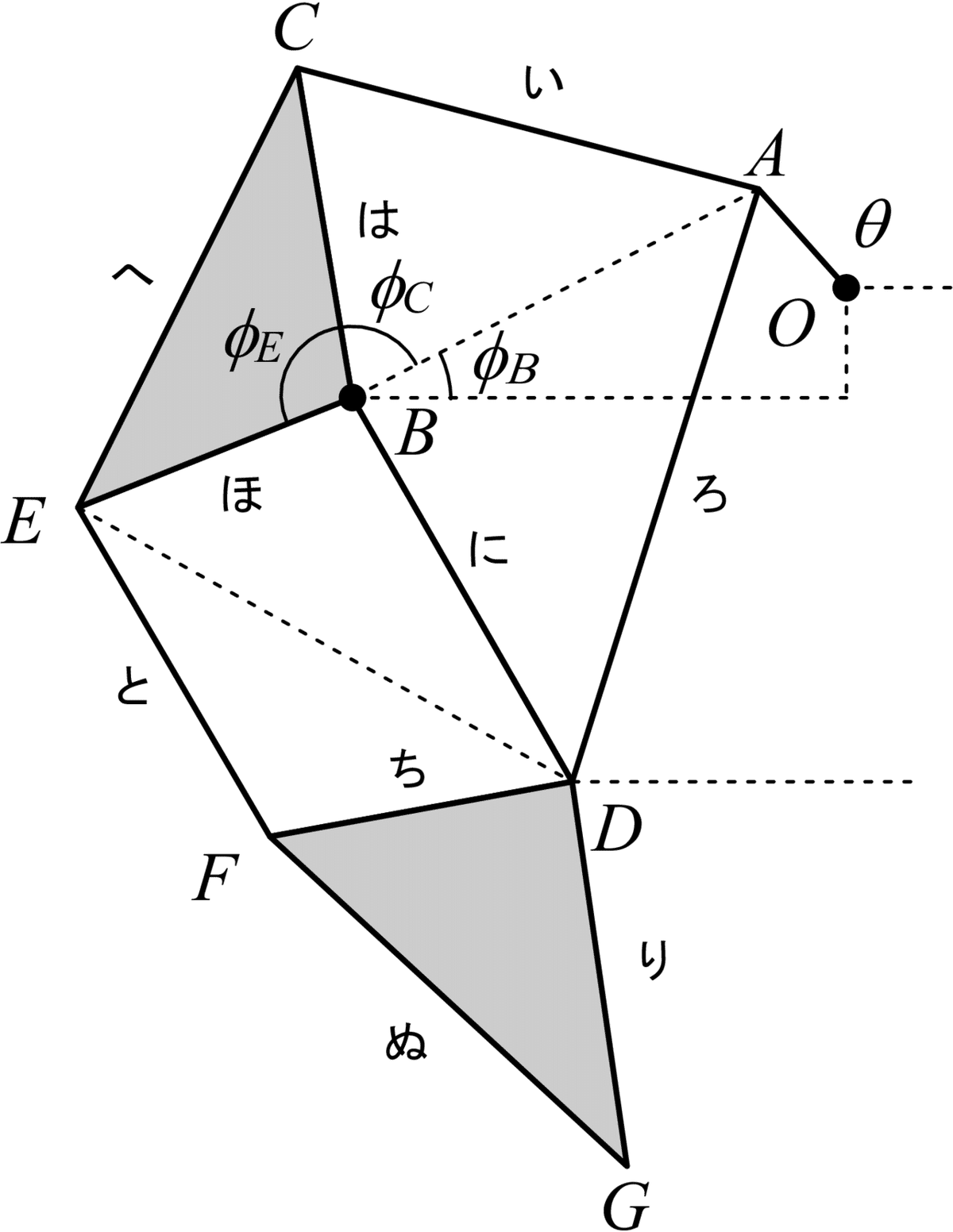
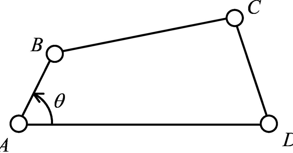
次に,点Cと点Eを求めます.ここで,下図のように3つの角度を定義します.余弦定理より,
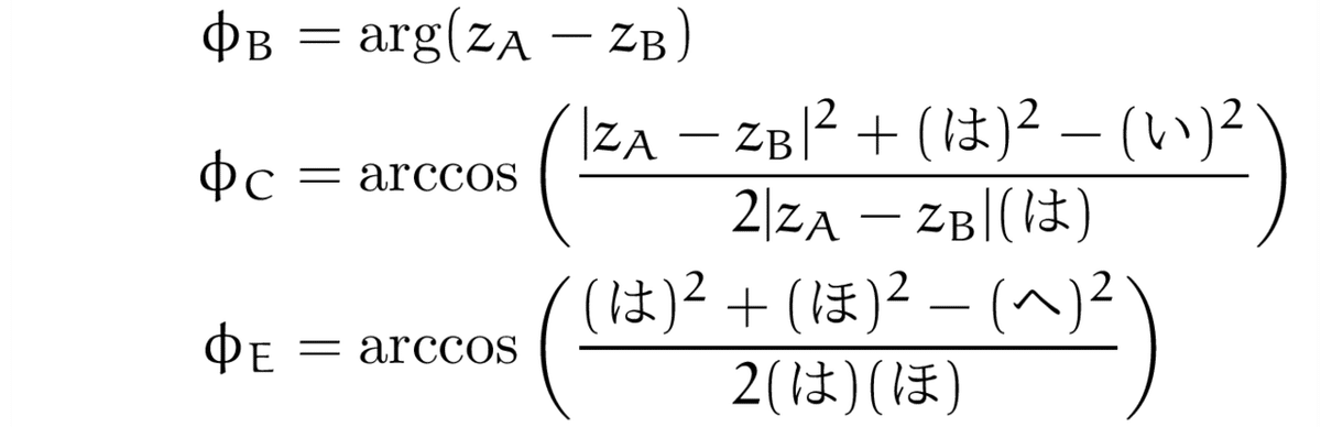
です.したがって,

となります.
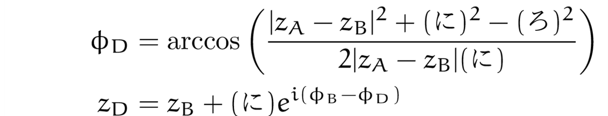
点Dの位置を求める
あとは,同様の作業を繰り返していくだけです.余弦定理よりΦDを求めます.
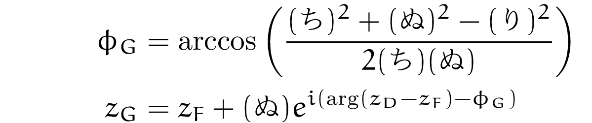
点F,点Gの位置を求める
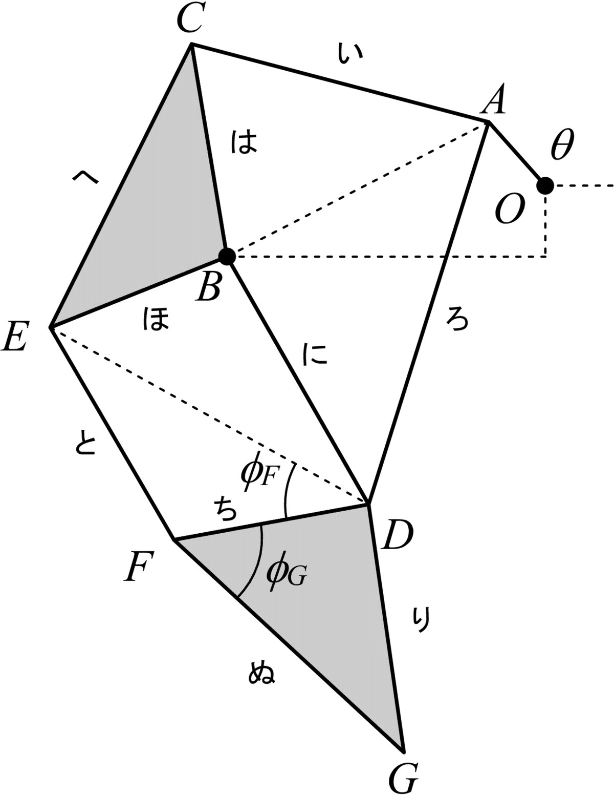
いよいよ面倒くさい式変形も最後です.点Fの偏角は,DEの偏角にΦFを加えたものですから,
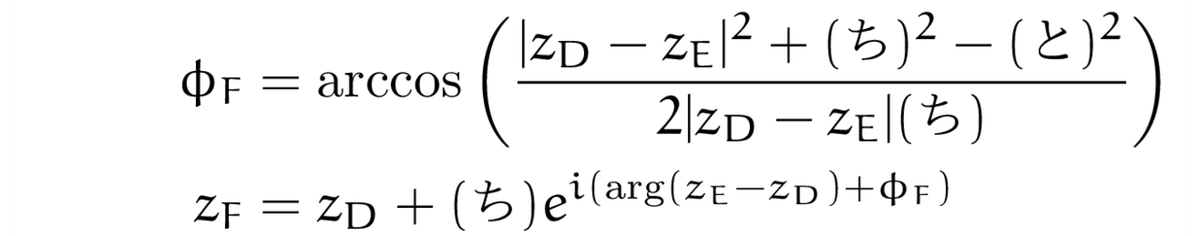
です.また,点Gの偏角は,FDの偏角からΦGを引いたものです.
コーディング with Python
以上でより得た数式を,あとはコーディングすればOKです.以下のソースコードはGoogle Colaboratory(Jupyter)での動作させることを前提としています.
はじめに,リンクの長さを定義します.
link_O = 15;    link_i = 50;    link_ro = 61.9; link_ha = 41.5
link_ni = 39.3; link_ho = 36.8; link_he = 53.2; link_to = 38.6
link_ti = 36.8; link_ri = 49;   link_nu = 65.7
先ほど求めた位置や角度を求めるメソッドを定義します.
omega = 1
def posA(t):
 return link_O * cmath.exp(1j*omega*t)

def posB(t=None):
 xb, yb = -38, -7.8
 return xb + yb*1j

def phiB(za, zb):
 return cmath.phase(za-zb)

def phiC(za, zb):
 AB = abs(za-zb)
 return np.arccos((AB**2+link_ha**2-link_i**2) / (2*AB*link_ha))

def posC(zb, pb, pc):
 return zb + link_ha * cmath.exp(1j*(pb + pc))

def phiD(za, zb):
 AB = abs(za-zb)
 return np.arccos((AB**2+link_ni**2-link_ro**2) / (2*AB*link_ni))

def posD(zb, pb, pd):
 return zb + link_ni * cmath.exp(1j*(pb-pd))

def phiE():
 return np.arccos((link_ha**2+link_ho**2-link_he**2) / (2*link_ha*link_ho))

def posE(zb, pb, pc, pe):
 return zb + link_ho * cmath.exp(1j*(pb+pc+pe))

def phiF(zd, ze):
 DE = abs(zd-ze)
 return np.arccos((DE**2+link_ti**2-link_to**2) / (2*DE*link_ti))

def posF(zd, ze, pf):
 arged = cmath.phase(ze-zd)
 return zd + link_ti * cmath.exp(1j*(arged + pf))

def phiG():
 return np.arccos((link_ti**2 + link_nu**2 - link_ri**2) / (2*link_ti*link_nu))

def posG(zd, zf, pg):
 argdf = cmath.phase(zd-zf)
 return zf + link_nu * cmath.exp(1j*(argdf - pg))
そして,それぞれの位置を配列を作ります.
N = 30
tl = np.linspace(2*np.pi, 0, N)
zOl = [0 + 0j for t in tl]
zal = [posA(t) for t in tl]
zbl = [posB() for t in tl]
pbl = [phiB(za, zb) for za, zb in zip(zal, zbl)]
pcl = [phiC(za, zb) for za, zb in zip(zal, zbl)]
zcl = [posC(zb, pb, pc) for zb, pb, pc in zip(zbl, pbl, pcl)]
pdl = [phiD(za, zb) for za, zb in zip(zal, zbl)]
zdl = [posD(zb, pb, pd) for zb, pb, pd in zip(zbl, pbl, pdl)]
pel = [phiE() for t in tl]
zel = [posE(zb, pb, pc, pe) for zb, pb, pc, pe in zip(zbl, pbl, pcl, pel)]
pfl = [phiF(zd, ze) for zd, ze in zip(zdl, zel)]
zfl = [posF(zd, ze, pf) for zd, ze, pf in zip(zdl, zel, pfl)]
pgl = [phiG() for t in tl]
zgl = [posG(zd, zf, pg) for zd, zf, pg in zip(zdl, zfl, pgl)]
プロットするメソッドを定義します.
def export_plot(index):
 filename = f"file{index:02d}.png"

 fig, ax = plt.subplots(figsize=(7,7))
 ax.axis('equal')

 lines = [
   [(zOl[index].real, zOl[index].imag), (zal[index].real, zal[index].imag)],  # link_O
   [(zal[index].real, zal[index].imag), (zcl[index].real, zcl[index].imag)],  # link_i
   [(zal[index].real, zal[index].imag), (zdl[index].real, zdl[index].imag)],  # link_ro
   [(zcl[index].real, zcl[index].imag), (zbl[index].real, zbl[index].imag)],  # link_ha
   [(zbl[index].real, zbl[index].imag), (zdl[index].real, zdl[index].imag)],  # link_ni
   [(zbl[index].real, zbl[index].imag), (zel[index].real, zel[index].imag)],  # link_ho
   [(zcl[index].real, zcl[index].imag), (zel[index].real, zel[index].imag)],  # link_he
   [(zel[index].real, zel[index].imag), (zfl[index].real, zfl[index].imag)],  # link_to
   [(zdl[index].real, zdl[index].imag), (zfl[index].real, zfl[index].imag)],  # link_ti
   [(zdl[index].real, zdl[index].imag), (zgl[index].real, zgl[index].imag)],  # link_ri
   [(zfl[index].real, zfl[index].imag), (zgl[index].real, zgl[index].imag)]   # link_nu
 ]

 col = mc.LineCollection(lines, linewidths=4)
 ax.set_xlim(-125, 25)
 ax.set_ylim(-100, 50)
 ax.add_collection(col)

 # 点対偶をプロット
 msize = 7
 ax.plot(zOl[index].real, zOl[index].imag, marker='o',
         markersize=msize, color='red')
 ax.plot(zbl[index].real, zbl[index].imag, marker='o',
         markersize=msize, color='red')

 points = [zal[index], zcl[index], zdl[index],
           zel[index], zfl[index], zgl[index]]
 for point in points:
   ax.plot(point.real, point.imag, marker='o',
           markersize=msize, color='blue')

 # 先端の奇跡をプロット
 x, y = [], []
 for zg in zgl:
   x.append(zg.real)
   y.append(zg.imag)
 ax.plot(x, y, linewidth=2, linestyle='dashed')

 ax.xaxis.set_visible(False)
 ax.yaxis.set_visible(False)

 fig.savefig(filename, bbox_inches='tight')  #, pad_inches=0)

 return filename
画像として出力します.そして,そのあと,APNGファイルにアニメーションとしてまとめます.Matplotlibの機能として,アニメーションとして出力することもできます.しかしながら,Google Collaboratory上での動作が安定しなかったため,「一度画像として出力したものを,APNGにまとめる」という方法を取りました.
files = []

for index in range(N):
 files.append(export_plot(index))

fps = 1/N
images = APNG.from_files(files, delay=int(fps*1000))
images.save('animation.png')
Google Collaboratory上でプレビューします.
IPython.display.Image(data=open("animation.png", 'rb').read(), format='png')
おわりに
一見複雑な機構ですが,使った数学は余弦定理だけとかなり単純に解くことができて驚きました.zGの座標を微分したりいろいろと式変形をすることで,地面を蹴る力Fと軸Oに必要となる回転トルクTも求めようかと思いましたが,それは†読者の演習問題†としたいと思います.
最後まで読んでいただきありがとうございました.したのColaboratoryからプログラムにアクセスしていろいろいじってみてください。書くリンクの長さや点Bの座標を変えることで,摩訶不思議な動きをするようになります.面白いパラメタの組を見つけたら教えてください.
記事の数式に誤りやタイポ,あるいはもっといいプログラミングの実装がありましたら,Twitter(@__yteshi)で教えていただけると幸いです.
この記事が気に入ったらサポートをしてみませんか?