
ゲームソフトの売上げ本数のデータを分析してみる3【python】

今回も引き続き、ゲームソフトの売り上げ本数のデータから調べてみようと思います。
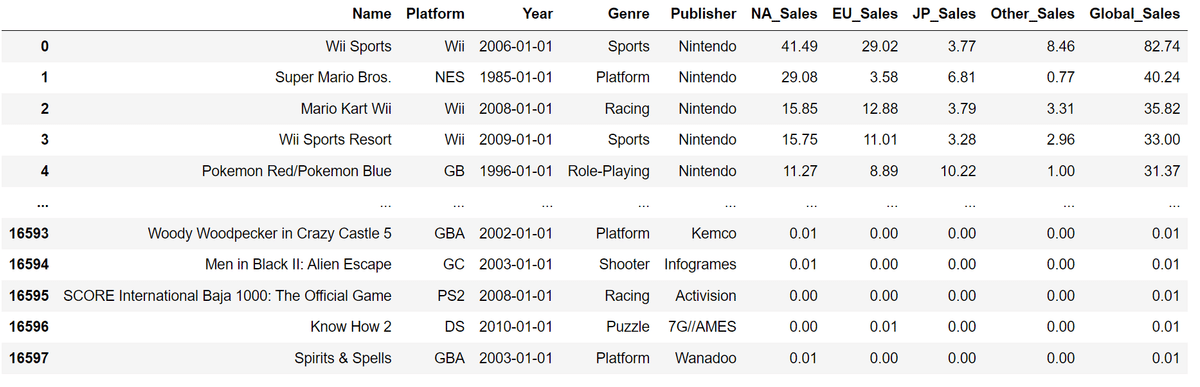
Jupyter Notebookでファイルを開きます。
import pandas as pd
df = pd.read_csv("C:\\Users\\csv_file\\vgsales.csv")    # csvファイルの読込
年代別に売上げ本数のデータをみます。
まずはdfを使えるように整形。
Nanが含まれているか確認します。
df.drop("Rank",axis=1,inplace=True)
df.isnull().sum()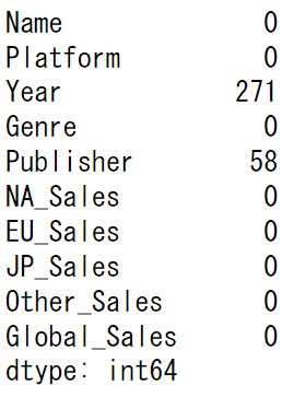
"Year"と"Publisher"の列にNan(Not a Number)が含まれているので、"Year"列に含まれているNanの行を削除します。
"Publisher"はNanでも問題ないので、そのままにします。
df.dropna(subset = ["Year"], inplace=True)
df.isnull().sum()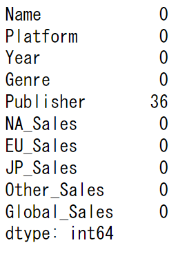
"Year"列のNanが0になりました。
次に"Year"のtypeをfloatからdatetimeに変更します。
df.dtypes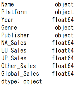
df["Year"] = pd.to_datetime(df['Year'],format='%Y')
df.dtypes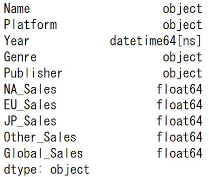
"Year"の列がdatestime型になって表示が変わりました。
Year
2006-01-01
1985-01-01
2008-01-01
年だけ分かれば十分なので月日は全て01-01で統一します。
datestime型にすると期間の指定ができます。
次は"Year"の列をindexにセットします。
df.set_index('Year', inplace=True)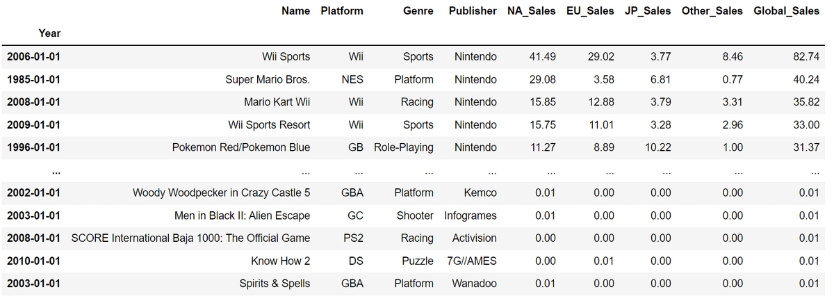
そして"Year"をグループ化して各Salesの数値を合計して、新たにdf_yearを作ります。
df_year = df.groupby("Year").sum()
df_year.head(10)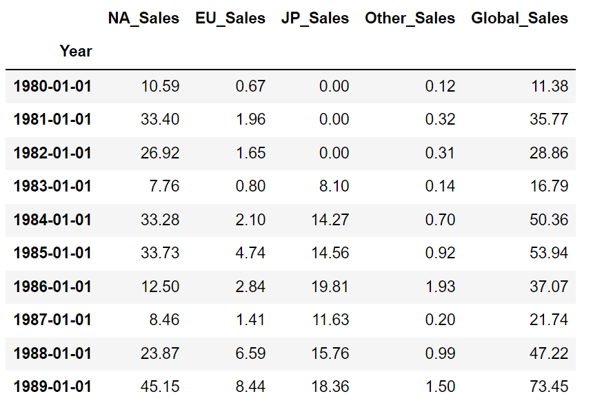
df_yearの"Global_Sales"を折れ線グラフで表します。
import matplotlib.pyplot as plt
fig, ax = plt.subplots()

ax.plot(df_year.index, df_year["Global_Sales"], label="Global_Sales")

plt.legend(fontsize=18)
plt.tick_params(labelsize=15)
fig.set_size_inches([8, 10])

plt.style.use('seaborn-darkgrid')
plt.show()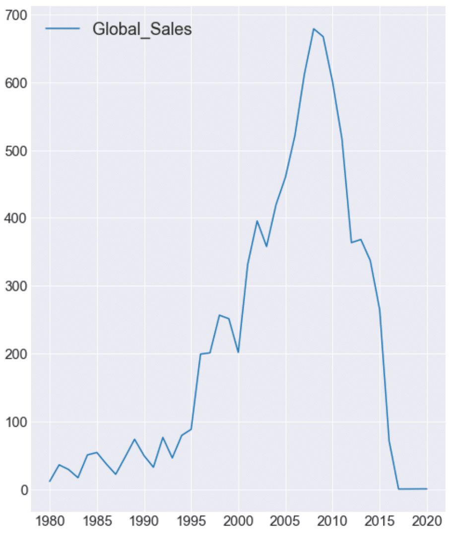
2000年から上がり続けてます。2002年で一度下がりますが、また上がって2008年ぐらいでピークを迎えてますね。
たしか、2000年はPlayStation 2が発売されて、2006年はPlayStation 3
とWiiが発売されました。その影響もあって7憶本近くのゲームソフトが売れてます。
2016年以降はデータが充分ではないため、"Global_Sales"が0に近い数値だったりします。
ではピーク辺りのグラフを見てみましょう。
期間を指定するために
df_year["2005-01-01":"2012-01-01"]と記述して変数ⅹに。
こうする事で、期間の変更が簡単にできます。
df_year["YYYY-MM-DD" :"YYYY-MM-DD"]
fig, ax = plt.subplots()

x = df_year["2005-01-01":"2012-01-01"]

ax.plot(x.index, x["Global_Sales"], label="Global_Sales")
plt.legend(fontsize=18)
plt.tick_params(labelsize=15)
fig.set_size_inches([8, 10])

plt.show()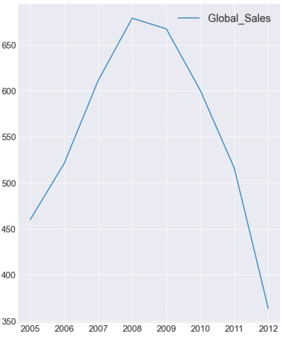
2007年から2010年までは、毎年6億本を超えて、2008年と2009年が6憶5千万越えです。それからグラフは下降してますね。
次は地域別にグラフを見ます。
fig, ax = plt.subplots()

ax.plot(df_year.index, df_year["NA_Sales"], label="NA_Sales")
ax.plot(df_year.index, df_year["EU_Sales"], label="EU_Sales")
ax.plot(df_year.index, df_year["JP_Sales"], label="JP_Sales")


plt.legend(fontsize=18)
plt.tick_params(labelsize=15)
fig.set_size_inches([8, 10])

plt.style.use('seaborn-darkgrid')
plt.show()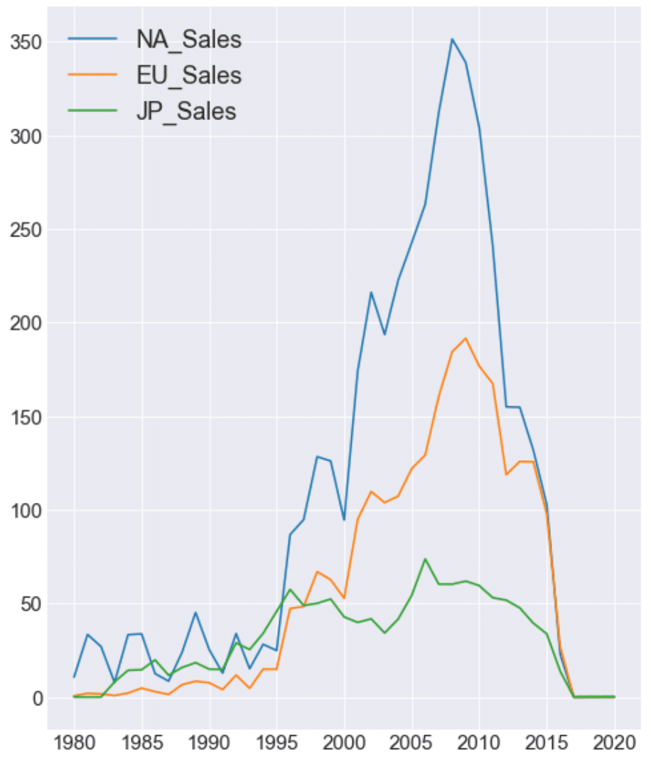
グラフにしてみると、ノースアメリカの市場の大きさがよく分かります。
2000年以降は、ヨーロッパの市場が伸びてますね。
90年代後半までは、日本市場の方がヨーロッパ市場より上だということが、興味深いです。
95年に初代PlayStationがヨーロッパで発売されて、ヨーロッパ市場で徐々に普及していったという感じでしょうか。
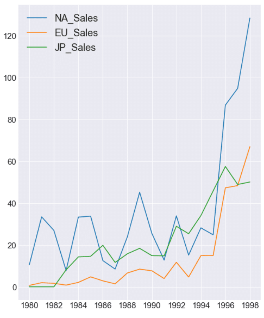
97年までは、緑色の”JP_Sales””がオレンジ色の”EU_Sales”より上にある。
今度は同じ年に発売されたPS3とWiiを比較してみましょう。
df_ps3 = df[df["Platform"] == "PS3"]
df_ps3_year = df_ps3.groupby("Year").sum()
df_ps3_year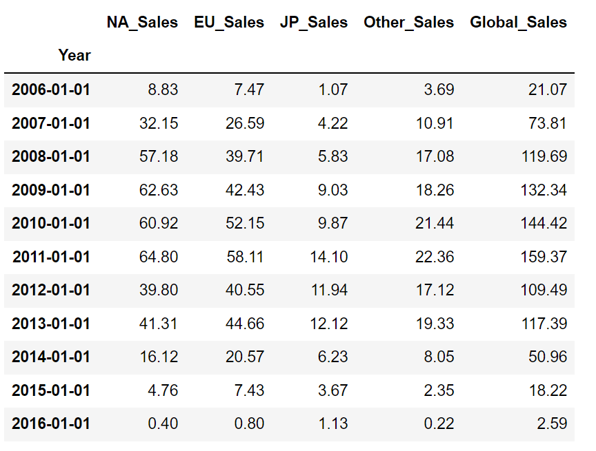
df_wii = df[df["Platform"] == "Wii"]
df_wii_year = df_wii.groupby("Year").sum()
df_wii_year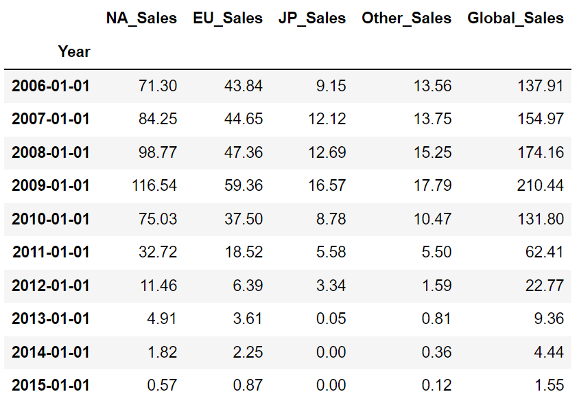
PS3とWiiのソフトの売上げ本数の比較。
fig, ax = plt.subplots()

ax.plot(df_ps3_year.index, df_ps3_year["Global_Sales"], label="PS3_Soft_Sales")
ax.plot(df_wii_year.index, df_wii_year["Global_Sales"], label="Wii_Soft_Sales")

plt.legend(fontsize=18)
plt.tick_params(labelsize=15)
fig.set_size_inches([8, 10])

plt.show()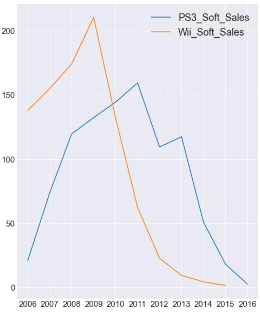
Wiiのゲームソフトは2009年をピークに2億本超えてます。
PS3のゲームソフトは2011年がピークで1億6千万本といったところでしょうか。
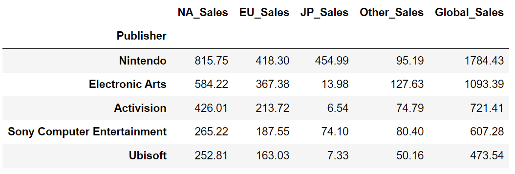
最後に各販売元のGlobal_SalesのTop5を見たいと思います。
df_ni = df[df["Publisher"] == "Nintendo"]
df_ni_year = df_ni.groupby("Year").sum()


df_ea = df[df["Publisher"] == "Electronic Arts"]
df_ea_year = df_ea.groupby("Year").sum()


df_ac = df[df["Publisher"] == "Activision"]
df_ac_year = df_ac.groupby("Year").sum()


df_sce = df[df["Publisher"] == "Sony Computer Entertainment"]
df_sce_year = df_sce.groupby("Year").sum()


df_ubi = df[df["Publisher"] == "Ubisoft"]
df_ubi_year = df_ubi.groupby("Year").sum()
fig, ax = plt.subplots()
ax.plot(df_ni_year.index, df_ni_year["Global_Sales"], label="Nintendo")
ax.plot(df_ea_year.index, df_ea_year["Global_Sales"], label="Electronic Arts")
ax.plot(df_ac_year.index, df_ac_year["Global_Sales"], label="Activision")
ax.plot(df_sce_year.index, df_sce_year["Global_Sales"], label="SCE")
ax.plot(df_ubi_year.index, df_ubi_year["Global_Sales"], label="UBI")
plt.legend(fontsize=18)
plt.tick_params(labelsize=15)
fig.set_size_inches([8, 10])
plt.show()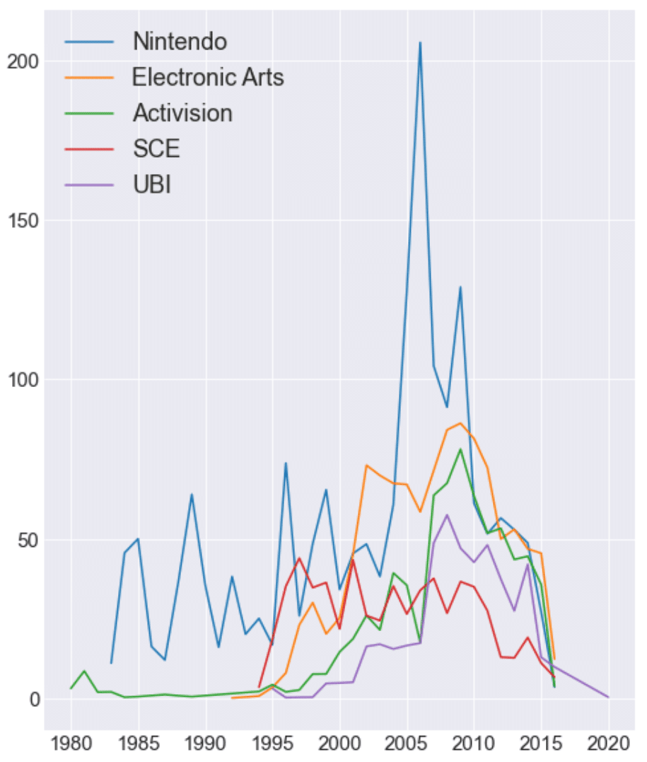
1位の任天堂のが圧倒的で、2005年から2010年までが飛び抜けてますね。
3位のActivisionが任天堂よりも、早くゲーム事業をしていた事に驚きです。
UBIとSCEは、同時期ぐらいにゲーム事業に参入していてますが、5年ぐらいUBIは低い位置にありますね。
2000年からはEAが大きく売れてます。
2010年以降は全体的に下降しています。
以上です。
この記事が気に入ったらサポートをしてみませんか?