小さな物体の検出率UPのためにSAHIを試してみた

概要
物体検出モデルが見逃しやすい小さな物体の検出力向上を目的としたライブラリSAHIを試してみました。
物体検出モデルにはYOLOv8sとYOLOv8xを使用しました。
YOLOのインスタンスセグメンテーションは未対応なようです。
SAHI (Slicing Aided Hyper Inference)
入力画像を分割して物体検出モデルに入力し、その結果をマージしてくれるライブラリです。
GitHubのGIFが視覚的にもわかりやすいです。
日本語での解説だと以下の記事がありました。
実施内容
Google ColabのT4環境で試しました。
比較といえるほどのことはしませんが、GitHubにあるテスト画像2枚とYOLOv8sとYOLOv8xの2モデルを試してみます。
精度の低いモデルと精度の高いモデルとでSAHIの効果の違いを見ようと考えました。
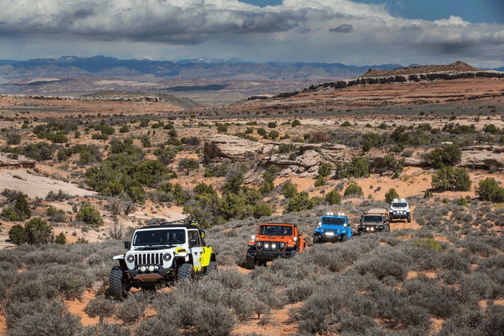
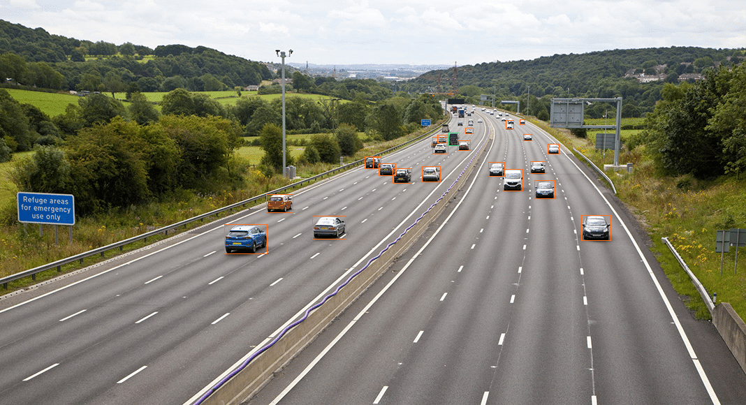
テスト画像①
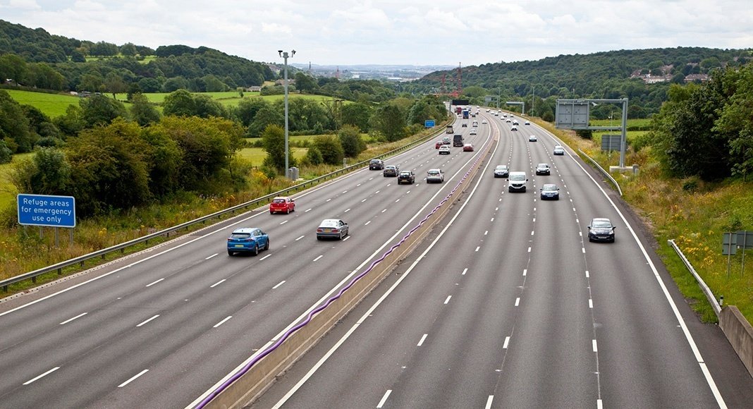
テスト画像②
準備
ライブラリをインストールします。
!pip install ultralytics sahi imantics fiftyoneインポートと資材のダウンロード
各種モジュールのインポートとテスト画像のダウンロードを行い、モデルのインスタンスを作成します。
from pathlib import Path

from IPython.display import Image
from sahi import AutoDetectionModel
from sahi.predict import get_prediction, get_sliced_prediction, predict
from sahi.utils.cv import read_image
from sahi.utils.file import download_from_url
from sahi.utils.yolov8 import download_yolov8s_model, download_yolov8x_model


# YOLOv8s & YOLOv8xの事前学習済みモデルをダウンロード
yolov8s_model_path = "yolov8s.pt"
yolov8x_model_path = "yolov8x.pt"
download_yolov8s_model(yolov8s_model_path)
download_yolov8x_model(yolov8x_model_path)

# テスト画像ダウンロード
download_from_url(
    "https://raw.githubusercontent.com/obss/sahi/main/demo/demo_data/small-vehicles1.jpeg",
    "small-vehicles1.jpeg",
)
download_from_url(
    "https://raw.githubusercontent.com/obss/sahi/main/demo/demo_data/terrain2.png",
    "terrain2.png",
)

# モデルのインスタンスを作成
detection_model_s = AutoDetectionModel.from_pretrained(
    model_type="yolov8",
    model_path=yolov8s_model_path,
    confidence_threshold=0.3,
    device="cuda:0",
)
detection_model_x = AutoDetectionModel.from_pretrained(
    model_type="yolov8",
    model_path=yolov8x_model_path,
    confidence_threshold=0.3,
    device="cuda:0",
)
通常の推論と結果の可視化
画像とモデルを get_prediction 関数に渡し、 通常通りの推論を実行します。
# sサイズの推論
s_result = get_prediction("small-vehicles1.jpeg", detection_model_s)
# xサイズの推論
x_result = get_prediction("small-vehicles1.jpeg", detection_model_x)
export_visuals メソッドで推論結果の可視化と保存を行います。
引数で保存先、保存するファイル名、矩形の枠の太さ、クラスラベルのON/OFF、confidenceスコアのON/OFFを指定できます。
# sサイズの推論結果を可視化&保存
s_result.export_visuals(export_dir="./", file_name="visualized_s_result", rect_th=1, hide_labels=True, hide_conf=True)
Image("visualized_s_result.png")  # 保存された画像をNotebookで表示
# xサイズの推論結果を可視化&保存
x_result.export_visuals(export_dir="./", file_name="visualized_x_result", rect_th=1, hide_labels=True, hide_conf=True)
Image("visualized_x_result.png")  # 保存された画像をNotebookで表示


スライス推論と結果の可視化
画像スライスを使用した推論は get_sliced_prediction 関数で行います。
画像とモデルに加えて、スライスのサイズ、オバーラップさせる比率、通常の推論も実行するか、後処理でカテゴリIDを無視するかなどを指定できます。
他にも指定可能な引数があるので、使用する際は該当関数のdocstringを確認してみてください。
# sサイズのスライス推論
s_sliced_result = get_sliced_prediction(
    "small-vehicles1.jpeg",
    detection_model_s,
    slice_height=128,
    slice_width=128,
    overlap_height_ratio=0.2,
    overlap_width_ratio=0.2,
    perform_standard_pred=False,
    postprocess_class_agnostic=True,
)
# xサイズのスライス推論
x_sliced_result = get_sliced_prediction(
    "small-vehicles1.jpeg",
    detection_model_x,
    slice_height=128,
    slice_width=128,
    overlap_height_ratio=0.2,
    overlap_width_ratio=0.2,
    perform_standard_pred=False,
    postprocess_class_agnostic=True,
)
先ほどと同様に結果を可視化して保存します。
# sサイズのスライス推論結果を可視化
s_sliced_result.export_visuals(export_dir="./", file_name="visualized_s_sliced_result", rect_th=1, hide_labels=True, hide_conf=True)
Image("visualized_s_sliced_result.png")  # 保存された画像をNotebookで表示
# xサイズのスライス推論結果を可視化
x_sliced_result.export_visuals(export_dir="./", file_name="visualized_x_sliced_result", rect_th=1, hide_labels=True, hide_conf=True)
Image("visualized_x_sliced_result.png")  # 保存された画像をNotebookで表示
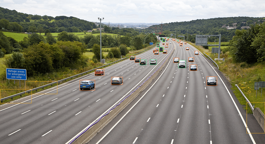
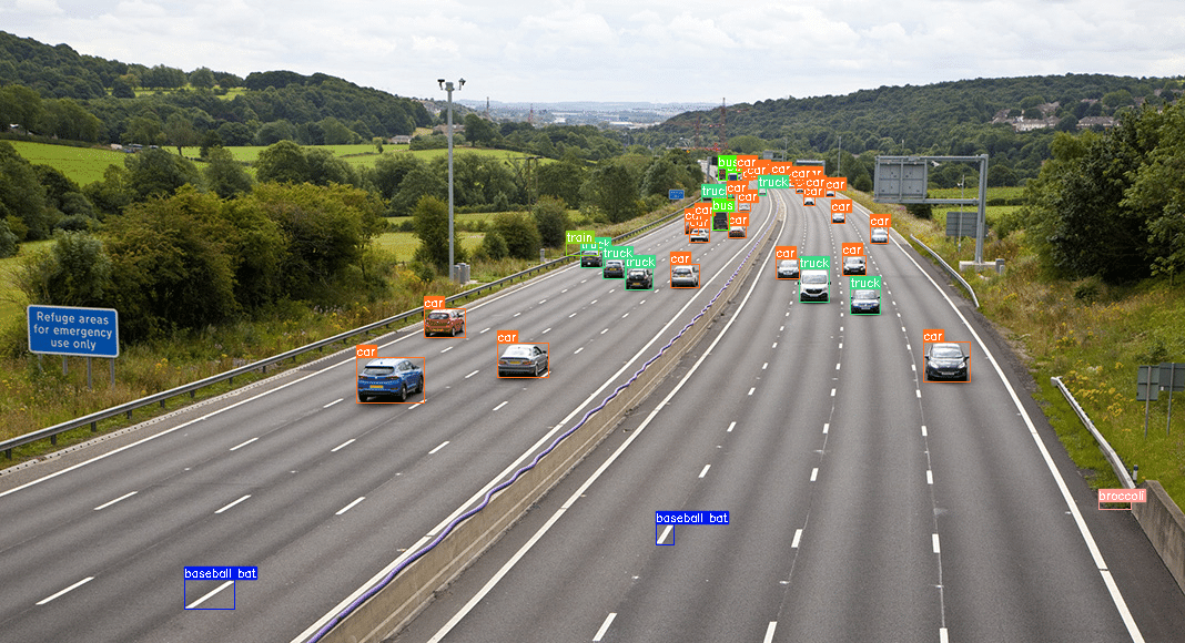
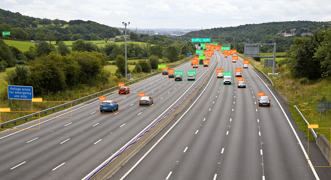
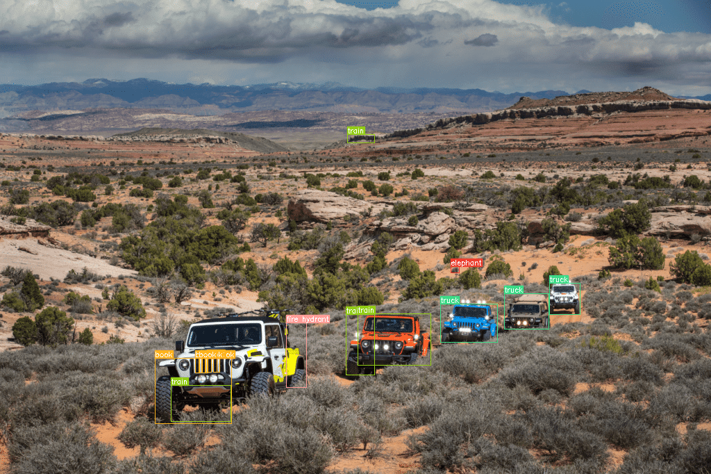
テスト画像①の結果を見ると、見逃しはあるものの小さな物体をしっかり検出できています。
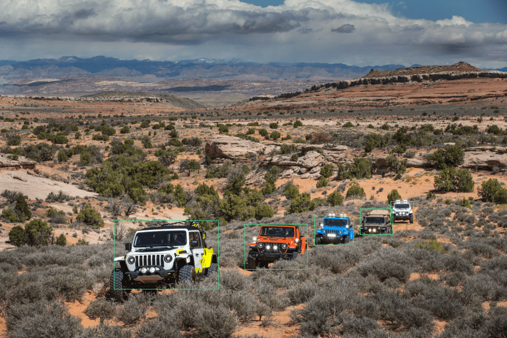
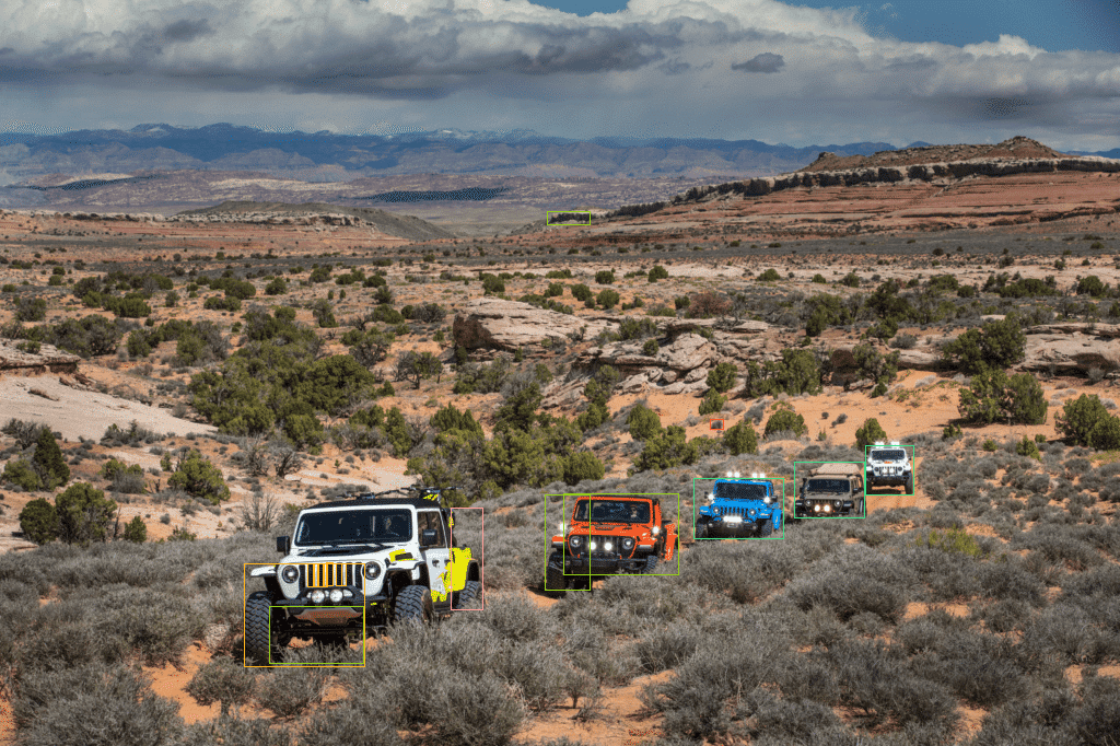
一方、物体が大きく映るテスト画像②はスライスがむしろ悪さをしたようで、車体の一部分を別のクラスとして検出したりしています。
上記の結果は get_sliced_prediction メソッド実行時にスライスサイズの引数 slice_height, slice_width で固定値を設定しました。
スライスサイズの指定を省略すると、解像度などから自動でスライスサイズを決定してくれます。
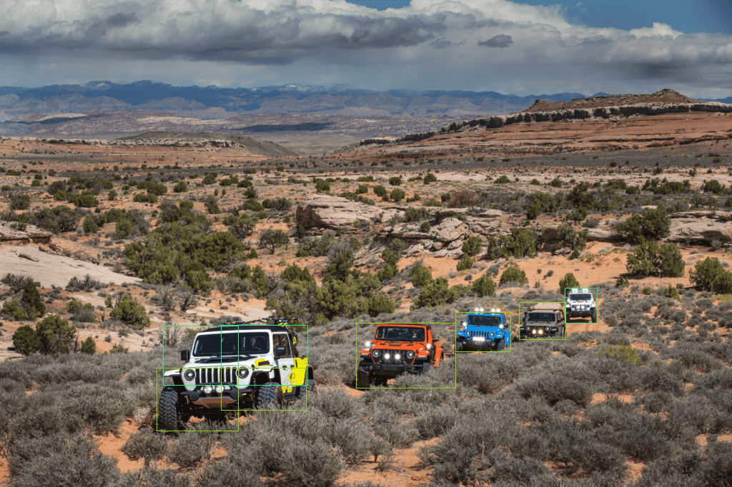
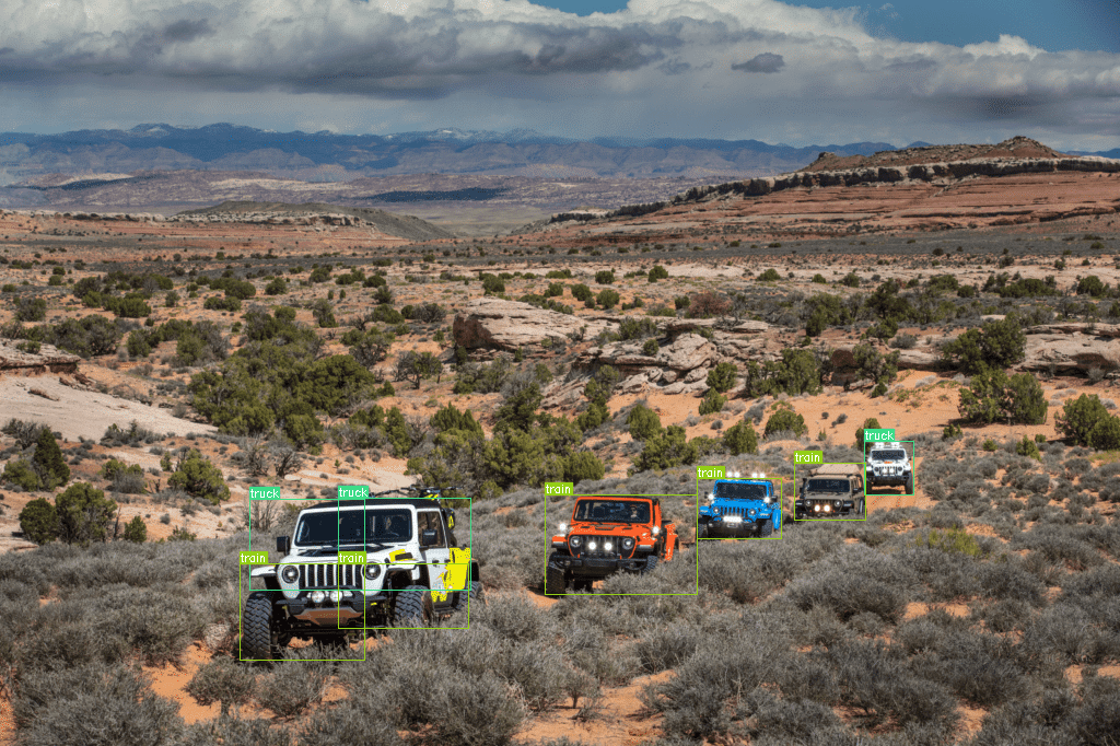
今回使用したテスト画像の場合は自動で6分割くらいになり、YOLOv8xの推論結果は下記の様になりました。
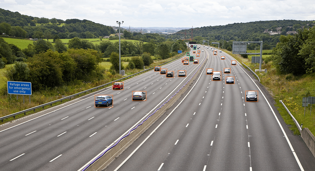


テスト画像②で発生していた車体の一部分を別のクラスにする問題は解消されていますが、テスト画像①の遠くの車の見逃しは増えてしまいました。
悩ましいですね…🤔
フォーマット変換
推論結果を変換可能なフォーマットもいくつか用意されています。
COCO形式くらいしか知らなかったので、「imantics?いえ、知らない子ですね…」と藤田咲さんボイスで脳内再生されました。
リスト
# ObjectPredictionクラスのリスト
object_prediction_list = s_sliced_result.object_prediction_list
object_prediction_list[:3]  # 最初の3件取得
[ObjectPrediction<
bbox: BoundingBox: <(448.26730728149414, 309.6943359375, 494.64769744873047, 340.30790519714355), w: 46.38039016723633, h: 30.613569259643555>,
mask: None,
score: PredictionScore: <value: 0.9161478281021118>,
category: Category: <id: 2, name: car>>,
ObjectPrediction<
bbox: BoundingBox: <(321.65446186065674, 322.37696838378906, 382.63111877441406, 363.1677360534668), w: 60.976656913757324, h: 40.790767669677734>,
mask: None,
score: PredictionScore: <value: 0.8996505737304688>,
category: Category: <id: 2, name: car>>,
ObjectPrediction<
bbox: BoundingBox: <(656.4625854492188, 203.19475555419922, 672.0792846679688, 214.93958377838135), w: 15.61669921875, h: 11.744828224182129>,
mask: None,
score: PredictionScore: <value: 0.856689989566803>,
category: Category: <id: 2, name: car>>]COCO annotation formats
# COCO annotation formats
s_sliced_result.to_coco_annotations()[:3][{'image_id': None,
'bbox': [448.26730728149414,
309.6943359375,
46.38039016723633,
30.613569259643555],
'score': 0.9161478281021118,
'category_id': 2,
'category_name': 'car',
'segmentation': [],
'iscrowd': 0,
'area': 1419},
{'image_id': None,
'bbox': [321.65446186065674,
322.37696838378906,
60.976656913757324,
40.790767669677734],
'score': 0.8996505737304688,
'category_id': 2,
'category_name': 'car',
'segmentation': [],
'iscrowd': 0,
'area': 2487},
{'image_id': None,
'bbox': [656.4625854492188,
203.19475555419922,
15.61669921875,
11.744828224182129],
'score': 0.856689989566803,
'category_id': 2,
'category_name': 'car',
'segmentation': [],
'iscrowd': 0,
'area': 183}]COCO prediction formats
# COCO prediction formats
s_sliced_result.to_coco_predictions(image_id=1)[:3][{'image_id': 1,
'bbox': [448.26730728149414,
309.6943359375,
46.38039016723633,
30.613569259643555],
'score': 0.9161478281021118,
'category_id': 2,
'category_name': 'car',
'segmentation': [],
'iscrowd': 0,
'area': 1419},
{'image_id': 1,
'bbox': [321.65446186065674,
322.37696838378906,
60.976656913757324,
40.790767669677734],
'score': 0.8996505737304688,
'category_id': 2,
'category_name': 'car',
'segmentation': [],
'iscrowd': 0,
'area': 2487},
{'image_id': 1,
'bbox': [656.4625854492188,
203.19475555419922,
15.61669921875,
11.744828224182129],
'score': 0.856689989566803,
'category_id': 2,
'category_name': 'car',
'segmentation': [],
'iscrowd': 0,
'area': 183}]imantics formats
# imantics formats
s_sliced_result.to_imantics_annotations()[:3][<imantics.annotation.Annotation at 0x7b7ba469d4b0>,
<imantics.annotation.Annotation at 0x7b7b95f4d1b0>,
<imantics.annotation.Annotation at 0x7b7b95f4d330>]fiftyone formats
# fiftyone formats
s_sliced_result.to_fiftyone_detections()[:3]
[<Detection: {
'id': '6658851da80c3d5f4494929a',
'attributes': {},
'tags': [],
'label': 'car',
'bounding_box': [
0.4197259431474664,
0.5339557516163793,
0.04342733161726248,
0.05278201596490268,
],
'mask': None,
'confidence': 0.9161478281021118,
'index': None,
}>,
<Detection: {
'id': '6658851da80c3d5f4494929b',
'attributes': {},
'tags': [],
'label': 'car',
'bounding_box': [
0.3011745897571692,
0.555822359282395,
0.057094248046589254,
0.07032890977530644,
],
'mask': None,
'confidence': 0.8996505737304688,
'index': None,
}>,
<Detection: {
'id': '6658851da80c3d5f4494929c',
'attributes': {},
'tags': [],
'label': 'car',
'bounding_box': [
0.6146653421809164,
0.35033578543827454,
0.014622377545646067,
0.020249703834796774,
],
'mask': None,
'confidence': 0.856689989566803,
'index': None,
}>]ソースを見ると bounding_box の要素は画像サイズで正規化された xywh のようです。
YOLO用データセットの形式で自動アノテーションしたい場合などはこちらを使うと良さそうですね!
所感
自動アノテーションに使えないかと思い試してみましたが、適切なスライスサイズの指定が必要なようなので、使うには工夫が必要そうです。
適切なスライスサイズが指定できれば小さな物体も結構検出できそうに感じました。
性能の高いモデルほどスライスの恩恵は薄くなりそうです。
自動アノテーションで使うための個人的な検討案
テスト画像①のbaseball batやbenchのような誤検出対策にアンサンブル的なことをする
GitHubのGIFの検出矩形が同色であることから想像すると、検出したい1クラスに特化したモデルでアノテーションする
補足
推論用の関数 get_prediction, get_sliced_prediction に画像のパスを指定しましたが、パスの代わりに画像の np.ndarray を指定することもできます。
また、実際に試していませんがバッチ推論の関数もあるようです。画像のディレクトリを指定してまとめて推論することもできそうです。
SAHIをYOLOv8のインスタンスセグメンテーションでも使用できないか試したりGitHubを眺めたりしましたが、現状はできなさそうです。
今回実施した内容は ultralyticsの記事 を参考にしました。
バッチ推論の関数
predict(
    model_type="yolov8",
    model_path="yolov8x.pt",
    model_device="cuda:0",
    model_confidence_threshold=0.4,
    source="./",
    slice_height=256,
    slice_width=256,
    overlap_height_ratio=0.2,
    overlap_width_ratio=0.2,
)この記事が気に入ったらサポートをしてみませんか?