
ブラックジャックを使った強化学習ライブラリGymnasiumのチュートリアル(2024年3月時点)

ChatGPTの学習でも使われている強化学習を勉強したいとずっと思っていたので、今回は実際に強化学習ライブラリを触ってみました。
完全に初心者なため、まずは強化学習ライブラリの現在の本命でありそうな"Gymnasium"の公式チュートリアルをそのままトレースし、ゆっくり理解することを目指したものです。
強化学習に関する日本語の情報は2024年の現在も自分が検索する限りでもそこまで多くない印象で、自分と同じように強化学習を触ってみたいなと思っている人の参考になればと思い、書いてみました。
間違っていることもあるかもしれませんが見つけたら優しくコメントください。
チュートリアルを選ぶにあたってどうせなら楽しいお題の方がいいので、こちらのブラックジャックのお題を選びました。今回はこのチュートリアルをほぼトレースしただけですので、英語をすんなり読める方はこちらの公式ページを進めていけば良いと思います。
※今回の実行環境はMac(Apple M2)です。
今回のチュートリアル上でのブラックジャックのルール

ブラックジャックの本来のルールは各自で調べてもらえればいいと思います。今回のチュートリアルで用意されているブラックジャックゲームは、簡素化されたものであり、ルールは以下のようになっています。なので強化学習での結果は実際のブラックジャックで勝てるようなものでは到底ありません。
デッキ枚数無限
ジャッククイーンキング絵札は"10"としてカウント
エースは11か1でカウント可能
ディーラー、プレイヤー双方に2枚のカードが配られ、ディーラーは1枚をプレイヤーに見せ、残りの1枚を伏せる。プレイヤーは自身の2枚の合計値を確認。
プレイヤーは合計値が21を超えるまでカードを要求可能。21を超えたらバーストとして強制的に負け。プレイヤーが追加カードを要求することを「ヒット」、要求終了を「ステイ」と呼ぶ。プレイヤーが要求終了時点で、ディーラーとプレイヤーで21に近い方が勝ち。
ディーラーはプレイヤーが要求終了時に伏せていたカードをオープンし、合計値が17を超えていない場合は、カードを追加しなければいけない。その際に21を超えた場合はディーラーのバースト負けである。
Gymnasiumのインストール

Gymnasiumのインストールはpipで簡単。今回はPython=3.10.12を使ってます。
# Python==3.10.12
pip install gymnasium
pip install matplotlib, seaborn, tqdm # 今回のチュートリアルで必要なライブラリ
ブラックジャックゲームの立ち上げ・ゲームスタート
ゲームの立ち上げ、ゲームスタートも非常に簡単です。
import gymnasium as gym

env = gym.make("Blackjack-v1")
observation, info = env.reset()
print(f"observation = {observation}")
>> observation = (9, 10, 0)
gym.make("Blackjack-v1")でゲームインスタンスを作成します。env.reset()でゲームを初期状態にします。このお作法は強化学習ライブラリの一般的なお作法みたいです。
observation変数がゲームスタート時の観測された状態です。(プレイヤーの手札合計値, ディーラーの表になっている1枚の値, プレイヤーの手札の中にエースがあるかどうか)の順で値が入っています。
上の例だと、「プレイヤーの手札合計値=9」「ディーラーの表になっている1枚の値=10」「プレイヤーの手札の中にエースがあるかどうか=ない」となります。
プレイヤーの行動を生成・その結果を反映
# sample a random action from all valid actions
action = env.action_space.sample()
print(f"action = {action}")
>> action = 1

# execute the action in our environment and receive infos from the environment
observation, reward, terminated, truncated, info = env.step(action)
print(f"observation = {observation}")
print(f"reward = {reward}")
print(f"terminated = {terminated}")
>> observation = (17, 10, 0)
>> reward = 0.0
>> terminated = False
env.action_space.sample()でプレイヤーの行動を生成します。今回、プレイヤーが選択できる行動は「ヒット(1)」か「ステイ(0)」のみです。なのでenv.action_space.sample()は0か1をランダムで返すだけです。今回は「1」が返ってきているため、プレイヤーはヒット(追加カードを要求)を選択しました。
env.action_space.sample()で生成したactionを受けてゲームを進めるのがenv.step(action)です。その結果がobservation, reward, terminated, truncatedなどに返ってきます。
observation: actionを受けた後の場の状態です。ゲームスタート時点での状態が(9, 10, 0)だったのが、(17, 10, 0)になりました。actionでヒットを要求したため、追加カードが与えられ、プレイヤーの合計値は17になりました。つまり8のカードを引いたことになりますね。
reward: プレイヤーが受け取る報酬です。勝ちで1、負けで-1が返ってきます。今回はまだ決着がついていませんので0が返ってきています。
terminated: 決着がついたかどうかのBoolean値です。まだ決着がついていませんのでFalseが返ってきています。
truncated/info: 今回truncatedとinfoは使用しないので無視します。
terminated=Trueが帰ってきた時点で1ゲーム終了です。その時のrewardがプレイヤーに与えられます。この報酬を最大化するために今回強化学習を使うことになります。
プレイヤーとディーラーの初期手札を確認する方法
チュートリアル上には記載されていませんがプレイヤーとディーラーの初期手札を確認することも可能です。env内に格納されています。前身のライブラリである"Gym"のソースコードを引き継いでいるようです。https://github.com/openai/gym/blob/master/gym/envs/toy_text/blackjack.py#L173-L174
env = gym.make("Blackjack-v1")
observation, info = env.reset()
player_hand = env.unwrapped.player
dealer_hand = env.unwrapped.dealer
print(f"observation = {observation}")
print(f"player's hand = {player_hand}")
print(f"dealer's hand = {dealer_hand}")

>> observation = (13, 1, 0)
>> player's hand = [5, 8]
>> dealer's hand = [1, 6] # 片方の1だけがobservationでは見えている状態
1ゲームの可視化
ここまでの内容で、1ゲームの流れをシミュレートすることができるようになりました。1ゲームの流れを少しわかりやすいように見える化してみようかと思います。
import gymnasium as gym
import pandas as pd


def simulate_1game():
    obs_list = []
    env = gym.make("Blackjack-v1")
    observation, info = env.reset()
    player_hand = env.unwrapped.player
    dealer_hand = env.unwrapped.dealer

    obs = {
        "player_hand": player_hand.copy(),
        "player_sum": observation[0],
        "dealer_opened_sum": observation[1],
        "dealer_hidden_card": dealer_hand.copy()[1],
    }
    obs_list.append(obs)

    done = False
    while not done:
        obs = {}
        action = env.action_space.sample()
        obs["action"] = action
        next_obs, reward, terminated, truncated, info = env.step(action)
        player_hand = env.unwrapped.player
        dealer_hand = env.unwrapped.dealer

        obs["player_hand"] = player_hand.copy()
        obs["player_sum"] = list(next_obs).copy()[0]
        obs["dealer_opened_sum"] = list(next_obs).copy()[1]
        obs["dealer_hidden_card"] = dealer_hand.copy()[1]

        obs["terminated"] = terminated
        obs["reward"] = reward

        if terminated:
            obs["dealer_final_hand"] = dealer_hand.copy()
        done = terminated
        obs_list.append(obs)

    simulate_df = pd.DataFrame.from_dict(obs_list)
    simulate_df = simulate_df[
        [
            "action",
            "player_hand",
            "player_sum",
            "dealer_opened_sum",
            "dealer_hidden_card",
            "terminated",
            "dealer_final_hand",
            "reward",
        ]
    ]
    return simulate_df


simulate_df = simulate_1game()
print(simulate_df)
上のコードを実行してもらうと下記のようなデータフレームができ、各ターンのカードの動きを確認することができます。

上記の例では、プレイヤーには最初に「6」「9」のカードが配られ合計値は15です。ディーラーの前には「2」のカードがオープンになっています。プレイヤーはまだ分かりませんがディーラーの伏せられているカードは10です。
1ターン目でプレイヤーはヒットを選択し、4のカードを引き、合計値を19にしました。
2ターン目でプレイヤーはステイを選択し、ディーラーが最初に伏せていた10がオープンになりました。ディーラーの合計値が17未満であるためディーラーは強制的に1枚カードを追加します。追加カードは10であったためディーラーがバーストし、プレイヤー側の勝利となり、報酬として1がプレイヤーに与えられました。
複数回シミュレーションを繰り返すと以下のような結果が生成されました。
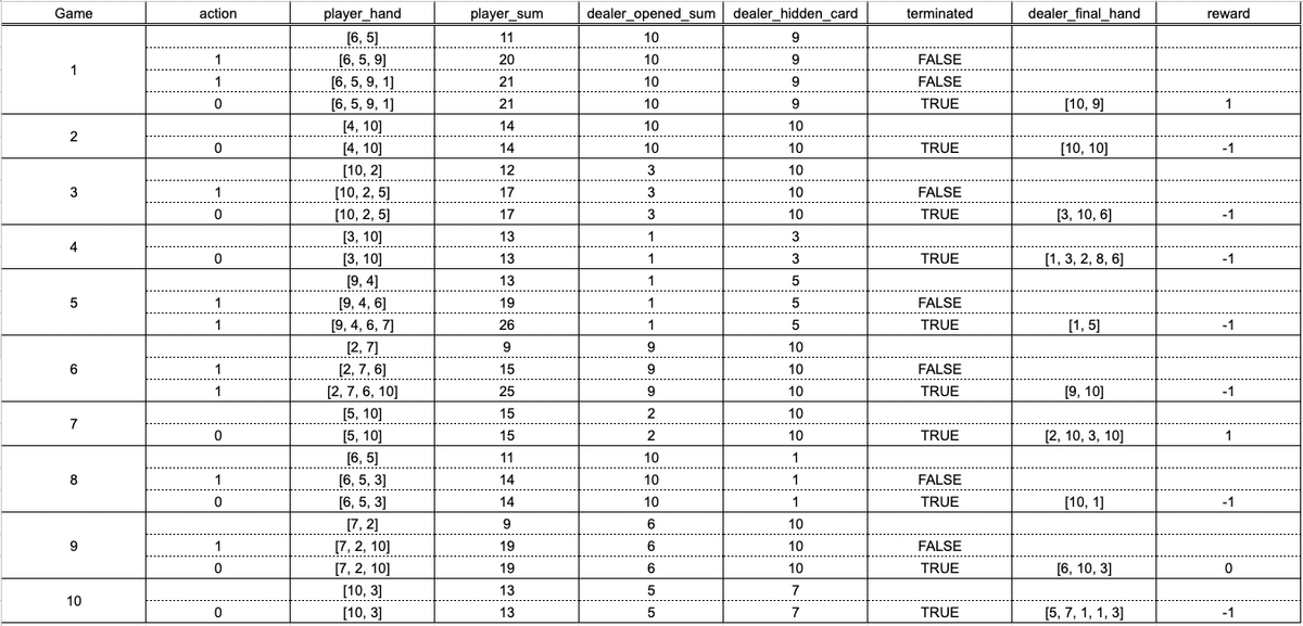
このシミュレーションを何回も回し最大の報酬が受け取れるように学習させていきたいところです。上記の例では負けの方が多いようですね。
さぁゲームの流れは把握できたので、本題の強化学習の部分に進みましょう
エージェントクラスの作成
ここが強化学習の本丸です。エージェントクラスを作成します。
強化学習においてエージェントとは行動を選択し、その行動によって報酬を受け取る対象のことを指します。つまり今回ではブラックジャックのプレイヤーということになりますね。
少し長いコードになりますが、ゆっくり理解していきたいと思います。
from collections import defaultdict
import numpy as np
import gymnasium as gym

env = gym.make("Blackjack-v1", sab=True)


class BlackjackAgent:
    def __init__(
        self,
        learning_rate: float,
        initial_epsilon: float,
        epsilon_decay: float,
        final_epsilon: float,
        discount_factor: float = 0.95,
    ):
        """Initialize a Reinforcement Learning agent with an empty dictionary
        of state-action values (q_values), a learning rate and an epsilon.

        Args:
            learning_rate: The learning rate
            initial_epsilon: The initial epsilon value
            epsilon_decay: The decay for epsilon
            final_epsilon: The final epsilon value
            discount_factor: The discount factor for computing the Q-value
        """
        self.q_values = defaultdict(lambda: np.zeros(env.action_space.n))

        self.lr = learning_rate
        self.discount_factor = discount_factor

        self.epsilon = initial_epsilon
        self.epsilon_decay = epsilon_decay
        self.final_epsilon = final_epsilon

        self.training_error = []

    def get_action(self, obs: tuple[int, int, bool]) -> int:
        """
        Returns the best action with probability (1 - epsilon)
        otherwise a random action with probability epsilon to ensure exploration.
        """
        # with probability epsilon return a random action to explore the environment
        if np.random.random() < self.epsilon:
            return env.action_space.sample()

        # with probability (1 - epsilon) act greedily (exploit)
        else:
            return int(np.argmax(self.q_values[obs]))

    def update(
        self,
        obs: tuple[int, int, bool],
        action: int,
        reward: float,
        terminated: bool,
        next_obs: tuple[int, int, bool],
    ):
        """Updates the Q-value of an action."""
        future_q_value = (not terminated) * np.max(self.q_values[next_obs])
        temporal_difference = reward + self.discount_factor * future_q_value - self.q_values[obs][action]

        self.q_values[obs][action] = self.q_values[obs][action] + self.lr * temporal_difference
        self.training_error.append(temporal_difference)

    def decay_epsilon(self):
        self.epsilon = max(self.final_epsilon, self.epsilon - self.epsilon_decay)
エージェントインスタンスが持つ初期値として以下が記載されています。
q_values: Q値。今回の学習方法はQ学習と呼ばれる手法で学習していきますが、Q学習はこのQ値を最大化するように学習します。Qテーブルとも呼ばれているみたいです。
lr: learning rate、学習率ですね。Q値の更新時にどれだけ新しい情報を取り入れるかを決めるパラメーターです。
discount_factor: 割引率と呼ばれるパラメーターです。将来もらえる報酬をどれくらい現在の価値として考慮に入れるかを表すパラメータです。少し難しい概念ですが、報酬を獲得するまでの過程の行動をどれだけ重視するかというパラメーターという理解を今はしています。
epsilon: これらはε-greedyアルゴリズムに関連するパラメータです。エージェントがランダムに行動を選ぶ確率(探索)と最適な行動を選ぶ確率(活用)のバランスを取ります。
この辺りのQ学習のパラメータに関しては詳しく解説してくれている記事などが勉強になりました。
エージェントインスタンスが持つメソッドの一つ目がget_action()です。これは分かりやすいですね。ヒットかステイかを選択しているだけですね。その際の確率としてε-greedyアルゴリズムによって制御されたepsilonが使われているのがポイントみたいです。毎回等確率でヒットかステイかを選択するわけではなく、ε-greedyアルゴリズムによって、ヒットかステイかを選ぶ確率は変動します。
2つ目のメソッドがupdate()で、各パラメータ周りを更新しています。
その中でTemporal Differenceというパラメータがありますが、これはTD誤差と言われている期待値(≈実際の報酬)と見込みの差分の誤差であり、TD誤差を使った学習のことをTD学習と呼ばれています。(つまりQ学習はTD学習の一部です)
学習開始
学習対象となるエージェントが作れたので、このエージェントのQ値を最大化できるように学習を回していきます。
# hyperparameters
learning_rate = 0.01
n_episodes = 100_000
start_epsilon = 1.0
epsilon_decay = start_epsilon / (n_episodes / 2)  # reduce the exploration over time
final_epsilon = 0.1

agent = BlackjackAgent(
    learning_rate=learning_rate,
    initial_epsilon=start_epsilon,
    epsilon_decay=epsilon_decay,
    final_epsilon=final_epsilon,
)

env = gym.wrappers.RecordEpisodeStatistics(env, deque_size=n_episodes)
for episode in tqdm(range(n_episodes)):
    obs, info = env.reset()
    done = False

    # play one episode
    while not done:
        action = agent.get_action(obs)
        next_obs, reward, terminated, truncated, info = env.step(action)

        # update the agent
        agent.update(obs, action, reward, terminated, next_obs)

        # update if the environment is done and the current obs
        done = terminated or truncated
        obs = next_obs

    agent.decay_epsilon()
episodeというのが1ゲームのことです。今回はエージェントに10万回のゲームを行ってもらい最大のQ値が得られる行動を探索しています。
学習過程の可視化
rolling_length = 500
fig, axs = plt.subplots(ncols=3, figsize=(12, 5))
axs[0].set_title("Episode rewards")
# compute and assign a rolling average of the data to provide a smoother graph
reward_moving_average = (
    np.convolve(
        np.array(env.return_queue).flatten(), np.ones(rolling_length), mode="valid"
    )
    / rolling_length
)
axs[0].plot(range(len(reward_moving_average)), reward_moving_average)
axs[1].set_title("Episode lengths")
length_moving_average = (
    np.convolve(
        np.array(env.length_queue).flatten(), np.ones(rolling_length), mode="same"
    )
    / rolling_length
)
axs[1].plot(range(len(length_moving_average)), length_moving_average)
axs[2].set_title("Training Error")
training_error_moving_average = (
    np.convolve(np.array(agent.training_error), np.ones(rolling_length), mode="same")
    / rolling_length
)
axs[2].plot(range(len(training_error_moving_average)), training_error_moving_average)
plt.tight_layout()
plt.show()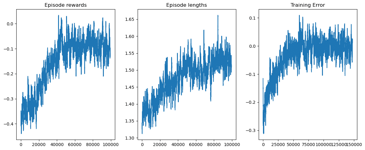
左: 1ゲームで得られた報酬の移動平均(500ゲーム)です。ゲーム回数が5万回くらいに至るまでは成長しており、それ以降は成長が止まっているようです。最終的に報酬がプラスに転じていることはないため、結果的にはこの学習方法では勝てないということになります。
中央: 1ゲームにおけるターン回数です。ターン回数とはつまりヒットのコール回数ですね、試行を重ねるたびにヒットのコール回数は増えていることを見ると、このエージェントはヒットは積極的に行った方が勝てる可能性が高いと学習したみたいです。
右: TD誤差のプロットです。報酬成長曲線もサチッてしまっているのと同様に誤差もサチってしまっており、ここらが限界という印象ですね。誤差がまだ縮まっていれば学習回数などを増やすことでまだ成長の余地はあると言えます。
ストラテジー表の作成
実際のブラックジャックにはストラテジー表というものが存在します。プレイヤーの手札のディラーの手札の組み合わせで、この時はこういう行動をしたらいいよ、と一目でわかる表です。要はパターン表ですね。
今回学習したエージェントからもこのストラテジー表を作成することができます。学習済みのエージェントインスタンスには各パターンのQ値が格納されているため、最大のQ値を取る行動を図にできます。
def create_grids(agent, usable_ace=False):
    """Create value and policy grid given an agent."""
    # convert our state-action values to state values
    # and build a policy dictionary that maps observations to actions
    state_value = defaultdict(float)
    policy = defaultdict(int)
    for obs, action_values in agent.q_values.items():
        state_value[obs] = float(np.max(action_values))
        policy[obs] = int(np.argmax(action_values))

    player_count, dealer_count = np.meshgrid(
        # players count, dealers face-up card
        np.arange(12, 22),
        np.arange(1, 11),
    )

    # create the value grid for plotting
    value = np.apply_along_axis(
        lambda obs: state_value[(obs[0], obs[1], usable_ace)],
        axis=2,
        arr=np.dstack([player_count, dealer_count]),
    )
    value_grid = player_count, dealer_count, value

    # create the policy grid for plotting
    policy_grid = np.apply_along_axis(
        lambda obs: policy[(obs[0], obs[1], usable_ace)],
        axis=2,
        arr=np.dstack([player_count, dealer_count]),
    )
    return value_grid, policy_grid


def create_plots(value_grid, policy_grid, title: str):
    """Creates a plot using a value and policy grid."""
    # create a new figure with 2 subplots (left: state values, right: policy)
    player_count, dealer_count, value = value_grid
    fig = plt.figure(figsize=plt.figaspect(0.4))
    fig.suptitle(title, fontsize=16)

    # plot the state values
    ax1 = fig.add_subplot(1, 2, 1, projection="3d")
    ax1.plot_surface(
        player_count,
        dealer_count,
        value,
        rstride=1,
        cstride=1,
        cmap="viridis",
        edgecolor="none",
    )
    plt.xticks(range(12, 22), range(12, 22))
    plt.yticks(range(1, 11), ["A"] + list(range(2, 11)))
    ax1.set_title(f"State values: {title}")
    ax1.set_xlabel("Player sum")
    ax1.set_ylabel("Dealer showing")
    ax1.zaxis.set_rotate_label(False)
    ax1.set_zlabel("Value", fontsize=14, rotation=90)
    ax1.view_init(20, 220)

    # plot the policy
    fig.add_subplot(1, 2, 2)
    ax2 = sns.heatmap(policy_grid, linewidth=0, annot=True, cmap="Accent_r", cbar=False)
    ax2.set_title(f"Policy: {title}")
    ax2.set_xlabel("Player sum")
    ax2.set_ylabel("Dealer showing")
    ax2.set_xticklabels(range(12, 22))
    ax2.set_yticklabels(["A"] + list(range(2, 11)), fontsize=12)

    # add a legend
    legend_elements = [
        Patch(facecolor="lightgreen", edgecolor="black", label="Hit"),
        Patch(facecolor="grey", edgecolor="black", label="Stick"),
    ]
    ax2.legend(handles=legend_elements, bbox_to_anchor=(1.3, 1))
    return fig


# state values & policy with usable ace (ace counts as 11)
value_grid, policy_grid = create_grids(agent, usable_ace=True)
fig1 = create_plots(value_grid, policy_grid, title="With usable ace")
plt.show()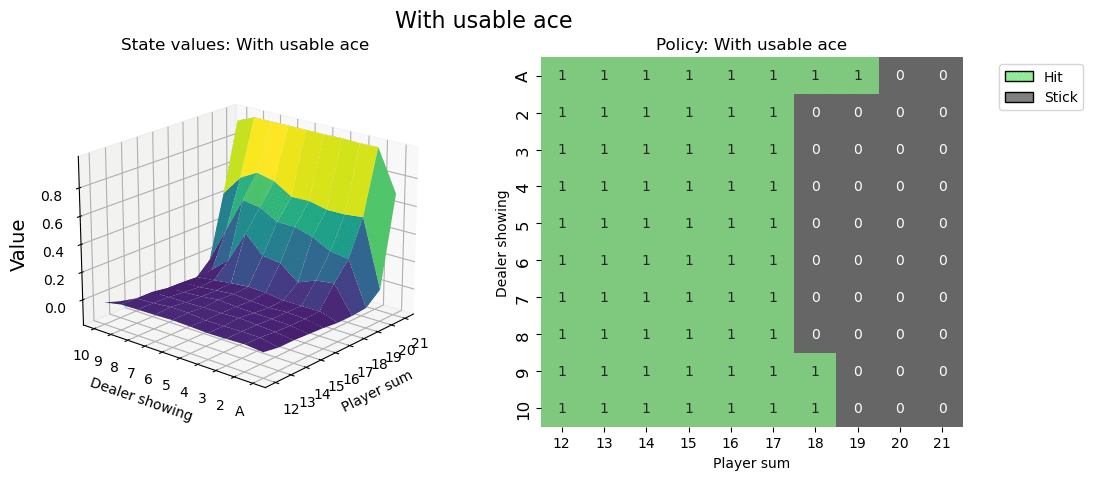
右の平面マトリックス図が、いわゆるストラテジー表です。横軸にプレイヤーの手札の合計値、縦軸にディラーの見えているカードになります。その時に1になっている部分が、今回学習したエージェントが最適解としてヒットすべきと提案しているパターンになります。逆に0の部分はステイです。(図ではStickという表記になっていますがステイと同義です)
左の3D図はz軸に報酬の期待値になります。プレイヤーの手札の合計値が高ければ高いほど勝利する期待値は高くなりますね。まぁ当然ではありますが。
以上、ブラックジャックを使った強化学習ライブラリGymnasiumのチュートリアルをゆっくりトレースしてみました。強化学習というものがどういうことをしようとしているか少しだけ理解ができた気がします。まだまだ初歩の初歩ですが、今後のための一歩になったかと思います。
最後に今回使用したコードの全体を記載しておきます。
コード全体
# Author: Till Zemann
# License: MIT License

from __future__ import annotations

from collections import defaultdict

import matplotlib.pyplot as plt
import numpy as np
import seaborn as sns
from matplotlib.patches import Patch
from tqdm import tqdm

import gymnasium as gym


# Let's start by creating the blackjack environment.
# Note: We are going to follow the rules from Sutton & Barto.
# Other versions of the game can be found below for you to experiment.

env = gym.make("Blackjack-v1", sab=True)

# reset the environment to get the first observation
done = False
observation, info = env.reset()

print(f"observation = {observation}")

# sample a random action from all valid actions
action = env.action_space.sample()
print(f"action = {action}")

# execute the action in our environment and receive infos from the environment
observation, reward, terminated, truncated, info = env.step(action)
print(f"observation = {observation}")
print(f"reward = {reward}")
print(f"terminated = {terminated}")
print(f"truncated = {truncated}")

# observation=(24, 10, False)
# reward=-1.0
# terminated=True
# truncated=False
# info={}


class BlackjackAgent:
    def __init__(
        self,
        learning_rate: float,
        initial_epsilon: float,
        epsilon_decay: float,
        final_epsilon: float,
        discount_factor: float = 0.95,
    ):
        """Initialize a Reinforcement Learning agent with an empty dictionary
        of state-action values (q_values), a learning rate and an epsilon.

        Args:
            learning_rate: The learning rate
            initial_epsilon: The initial epsilon value
            epsilon_decay: The decay for epsilon
            final_epsilon: The final epsilon value
            discount_factor: The discount factor for computing the Q-value
        """
        self.q_values = defaultdict(lambda: np.zeros(env.action_space.n))

        self.lr = learning_rate
        self.discount_factor = discount_factor

        self.epsilon = initial_epsilon
        self.epsilon_decay = epsilon_decay
        self.final_epsilon = final_epsilon

        self.training_error = []

    def get_action(self, obs: tuple[int, int, bool]) -> int:
        """
        Returns the best action with probability (1 - epsilon)
        otherwise a random action with probability epsilon to ensure exploration.
        """
        # with probability epsilon return a random action to explore the environment
        if np.random.random() < self.epsilon:
            return env.action_space.sample()

        # with probability (1 - epsilon) act greedily (exploit)
        else:
            return int(np.argmax(self.q_values[obs]))

    def update(
        self,
        obs: tuple[int, int, bool],
        action: int,
        reward: float,
        terminated: bool,
        next_obs: tuple[int, int, bool],
    ):
        """Updates the Q-value of an action."""
        future_q_value = (not terminated) * np.max(self.q_values[next_obs])
        temporal_difference = reward + self.discount_factor * future_q_value - self.q_values[obs][action]

        self.q_values[obs][action] = self.q_values[obs][action] + self.lr * temporal_difference
        self.training_error.append(temporal_difference)

    def decay_epsilon(self):
        self.epsilon = max(self.final_epsilon, self.epsilon - self.epsilon_decay)


# hyperparameters
learning_rate = 0.01
n_episodes = 100_000
start_epsilon = 1.0
epsilon_decay = start_epsilon / (n_episodes / 2)  # reduce the exploration over time
final_epsilon = 0.1

agent = BlackjackAgent(
    learning_rate=learning_rate,
    initial_epsilon=start_epsilon,
    epsilon_decay=epsilon_decay,
    final_epsilon=final_epsilon,
)


env = gym.wrappers.RecordEpisodeStatistics(env, deque_size=n_episodes)
for episode in tqdm(range(n_episodes)):
    obs, info = env.reset()
    done = False

    # play one episode
    while not done:
        action = agent.get_action(obs)
        next_obs, reward, terminated, truncated, info = env.step(action)

        # update the agent
        agent.update(obs, action, reward, terminated, next_obs)

        # update if the environment is done and the current obs
        done = terminated or truncated
        obs = next_obs

    agent.decay_epsilon()


rolling_length = 500
fig, axs = plt.subplots(ncols=3, figsize=(12, 5))
axs[0].set_title("Episode rewards")
# compute and assign a rolling average of the data to provide a smoother graph
reward_moving_average = (
    np.convolve(np.array(env.return_queue).flatten(), np.ones(rolling_length), mode="valid") / rolling_length
)
axs[0].plot(range(len(reward_moving_average)), reward_moving_average)
axs[1].set_title("Episode lengths")
length_moving_average = (
    np.convolve(np.array(env.length_queue).flatten(), np.ones(rolling_length), mode="same") / rolling_length
)
axs[1].plot(range(len(length_moving_average)), length_moving_average)
axs[2].set_title("Training Error")
training_error_moving_average = (
    np.convolve(np.array(agent.training_error), np.ones(rolling_length), mode="same") / rolling_length
)
axs[2].plot(range(len(training_error_moving_average)), training_error_moving_average)
plt.tight_layout()
plt.show()


def create_grids(agent, usable_ace=False):
    """Create value and policy grid given an agent."""
    # convert our state-action values to state values
    # and build a policy dictionary that maps observations to actions
    state_value = defaultdict(float)
    policy = defaultdict(int)
    for obs, action_values in agent.q_values.items():
        state_value[obs] = float(np.max(action_values))
        policy[obs] = int(np.argmax(action_values))

    player_count, dealer_count = np.meshgrid(
        # players count, dealers face-up card
        np.arange(12, 22),
        np.arange(1, 11),
    )

    # create the value grid for plotting
    value = np.apply_along_axis(
        lambda obs: state_value[(obs[0], obs[1], usable_ace)],
        axis=2,
        arr=np.dstack([player_count, dealer_count]),
    )
    value_grid = player_count, dealer_count, value

    # create the policy grid for plotting
    policy_grid = np.apply_along_axis(
        lambda obs: policy[(obs[0], obs[1], usable_ace)],
        axis=2,
        arr=np.dstack([player_count, dealer_count]),
    )
    return value_grid, policy_grid


def create_plots(value_grid, policy_grid, title: str):
    """Creates a plot using a value and policy grid."""
    # create a new figure with 2 subplots (left: state values, right: policy)
    player_count, dealer_count, value = value_grid
    fig = plt.figure(figsize=plt.figaspect(0.4))
    fig.suptitle(title, fontsize=16)

    # plot the state values
    ax1 = fig.add_subplot(1, 2, 1, projection="3d")
    ax1.plot_surface(
        player_count,
        dealer_count,
        value,
        rstride=1,
        cstride=1,
        cmap="viridis",
        edgecolor="none",
    )
    plt.xticks(range(12, 22), range(12, 22))
    plt.yticks(range(1, 11), ["A"] + list(range(2, 11)))
    ax1.set_title(f"State values: {title}")
    ax1.set_xlabel("Player sum")
    ax1.set_ylabel("Dealer showing")
    ax1.zaxis.set_rotate_label(False)
    ax1.set_zlabel("Value", fontsize=14, rotation=90)
    ax1.view_init(20, 220)

    # plot the policy
    fig.add_subplot(1, 2, 2)
    ax2 = sns.heatmap(policy_grid, linewidth=0, annot=True, cmap="Accent_r", cbar=False)
    ax2.set_title(f"Policy: {title}")
    ax2.set_xlabel("Player sum")
    ax2.set_ylabel("Dealer showing")
    ax2.set_xticklabels(range(12, 22))
    ax2.set_yticklabels(["A"] + list(range(2, 11)), fontsize=12)

    # add a legend
    legend_elements = [
        Patch(facecolor="lightgreen", edgecolor="black", label="Hit"),
        Patch(facecolor="grey", edgecolor="black", label="Stick"),
    ]
    ax2.legend(handles=legend_elements, bbox_to_anchor=(1.3, 1))
    return fig


# state values & policy with usable ace (ace counts as 11)
value_grid, policy_grid = create_grids(agent, usable_ace=True)
fig1 = create_plots(value_grid, policy_grid, title="With usable ace")
plt.show()

# state values & policy without usable ace (ace counts as 1)
value_grid, policy_grid = create_grids(agent, usable_ace=False)
fig2 = create_plots(value_grid, policy_grid, title="Without usable ace")
plt.show()この記事が気に入ったらサポートをしてみませんか?