
New Method for Solving the Collatz Conjecture 6 with High-Prize Money

Chapter 5: Chaos Dynamics 1D Mapping
(article 6)
Please read "Introduction to a New Method in Chapter 1 (article 1)"
before reading Chapter 5 (article 6).
Chapter 1 also posts links to each chapter.
When translating from Japanese to English, subtle nuances of the original articles may not be fully conveyed. If you would like to view the original Japanese articles, please see Chapter 1 of Japanese Article 1.
Summary Video of the New Method in English
5.1 Similarity between the Collatz Conjecture (CS-Space)
and 1D Mapping
Consider an infinite sequence of coin tosses, where heads is represented by A and tails by B. This can be arranged infinitely, resulting in an infinite number of arrangements. (The probability of each sequence can be calculated using the principles of probability theory. However, the focus here is not on the probabilities.)
Examples of infinite sequences:
$${AABABBABBAA\cdots}$$
$${BABAABBABAA\cdots}$$
There are an infinite number of such patterns.
A fascinating discovery in chaos theory is that
any pattern can be expressed depending on the initial value
by using a simple one-dimensional map $${f(x)}$$.
It was quite shocking when I first learned about it
In that case, by assigning A to prime numbers and B to composite numbers in ascending order from 1, the prime number pattern can also be determined, once an initial value is determined.
For examples of A and B, refer to Figure 5-2.
Readers who are working on solving the Collatz conjecture, including myself, tend to get hooked on things. There is a high probability that we will also be fascinated by this chaotic one-dimensional map. It may even lead to the elucidation of prime numbers, which is the pinnacle of mathematics.
If that happens, it will be more than just solving the Collatz conjecture.
A single one-dimensional map, $${f(x)}$$, can generate any pattern.
For a sequence $${\{x_0, x_1, x_2, \cdots, x_n, x_{n+1}, \cdots\}}$$,
depending on the initial value $${x_0}$$,
(a) It can generate a sequence where all values are different,.
(b) It can generate any periodic sequence, such as those with periods of 2
$${abab\cdots}$$, 3 $${abcabc\cdots}$$, and so on.
(c) It can also generate a sequence that converges to a specific value.
Indeed, this must be a clue to solving the Collatz conjecture.
(a) corresponds to the case where a sequence following the Collatz rule goes to infinity somewhere.
(b) corresponds to the case where a sequence returns to a certain number.
(c) corresponds to the case where a sequence reaches 1.
The new method is a technique in a world where the number sequence of the general Collatz space is converted to a value between 0 and 1, and it enables the use of the theory of chaotic one-dimensional maps.
Chaotic one-dimensional maps can be a fascinating area of study, and I hope you will consider applying this new method to your research. It may provide a valuable clue towards solving the Collatz conjecture.
This new method is only an introductory part. At the same time, you may also come up with hints for solving the prime number problem.
Although other researchers are working on this topic, as you can see by searching for "Collatz" and "chaos," this new method is completely different.
The images in Figure 5-1 (center and right) that have already been introduced cannot be found anywhere else except in this note article, even with a Google keyword search.

The right image shows that the plot points are located near the CS-line.
For a perfectly matched image, please refer to Figure 4-1 in Chapter 4.
The properties of one-dimensional maps are used in the introduction of the new method, so they are presented in Chapter 5 as a separate chapter, similar to Chapter 3.
The Lorenz plot is relevant to the new method, and understanding it is essential for understanding the new method. Therefore, this chapter will only introduce a few examples of this plot.
There are proofs that any pattern can be represented using the aforementioned method, and that the sequence becomes infinite if the initial value is irrational, and so on. However, these topics are beyond the scope of this article, so please refer to other websites for more information.
5.2 Tent Map (Example of 1D Mapping) change of pace
This section introduces the tent map, which is an example of a one-dimensional map. The tent map is defined by the following equation:
$${ ax (A:0 \le x \le 1/2)}$$
$${(5.1) f(x)=}$$
$${ a(1-x) (B:1/2 < x \le 1)}$$
Figure 5-2 shows the tent map with $${a=2}$$. The line $${y=x}$$ is an auxiliary line to help visualize the Lorenz plot.
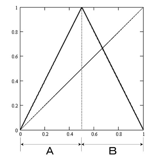
Consider a sequence $${\{x_0, x_1, x_2, \cdots, x_n, x_{n+1}, \cdots\}}$$ where $${x_{n+1}}$$ depends only on $${x_n}$$, i.e. $${x_{n+1}=f(x_n)}$$
The sequence can be represented by the composite function as:
$${\{x_0, f(x_0),f^2( x_0), \cdots, f^n(x_0), f^{n+1}(x_0), \cdots\}}$$
where $${f^2( x_0)=f(f( x_0))}$$ and so on.
The horizontal axis shows the values of $${x_n}$$ and the vertical axis shows the values of $${x_{n+1}}$$. In other words, the points $${(x_n, x_{n+1})}$$ are plotted for $${n=0,1,2,3,\cdots }$$ in sequence. This is called a Lorenz plot and is one of the methods of chaos analysis.
Consider the following example:
Case $${x_0=\cfrac{1}{3}}$$ :
The sequence generated from Equation (5.1) with the initial value $${x_0=\cfrac{1}{3}}$$
is:
$${\left\{\cfrac{1}{3}, \cfrac{2}{3}, \cfrac{2}{3},\cdots\right\}}$$ (a)
The Lorenz plot for this sequence is:
$${\left(\cfrac{1}{3}, \cfrac{2}{3}\right), \left(\cfrac{2}{3}, \cfrac{2}{3}\right), \left(\cfrac{2}{3}, \cfrac{2}{3}\right), \cdots}$$
Case$${x_0=\cfrac{1}{10}}$$ :
The sequence generated from Equation (5.1) with the initial value $${x_0=\cfrac{1}{10}}$$ is:
$${\left\{\cfrac{1}{10}, \cfrac{1}{5}, \cfrac{2}{5}, \cfrac{4}{5},\cfrac{2}{5}, \cfrac{4}{5},\cdots\right\}}$$ (b)
The corresponding Lorenz plot is:
$${\left(\cfrac{1}{10}, \cfrac{1}{5}\right), \left(\cfrac{1}{5}, \cfrac{2}{5}\right), \left(\cfrac{2}{5}, \cfrac{4}{5}\right),\left(\cfrac{4}{5}, \cfrac{2}{5}\right), \cdots}$$
(a) is the orbit with the initial $${\cfrac{1}{3}}$$ and is called a one-period orbit.
(b) is the orbit with the initial value $${\cfrac{1}{10}}$$ and is called a two-period orbit.
Here, the points $${\cfrac{1}{3}}$$, $${\cfrac{1}{5}}$$, and $${\cfrac{1}{10}}$$ are not periodic points. Instead, they are called eventually periodic points.
The Lorenz plot for (a) is shown in the left figure of Figure 5-3, and the Lorenz plot for (b) is shown in the right figure.
The initial value $${x_0}$$ is taken as $${(x_0,0)}$$ on the x-axis.
Instead of connecting the Lorenz plot points directly, the vertical and horizontal lines shown by the arrows are used to visualize the movement via the point on $${y=x}$$. This method is called the cobweb diagram.
In the right figure, the trajectory eventually becomes an orbit that oscillates infinitely between the points $${x_2}$$ and $${x_3}$$ on the x-axis. However, in the cobweb diagram, the two points ● on the tent map can be seen as rotating via $${y=x}$$, which makes it easier to see the periodicity.

The following are the methods for finding 1-periodic, 2-periodic, and 3-periodic points.
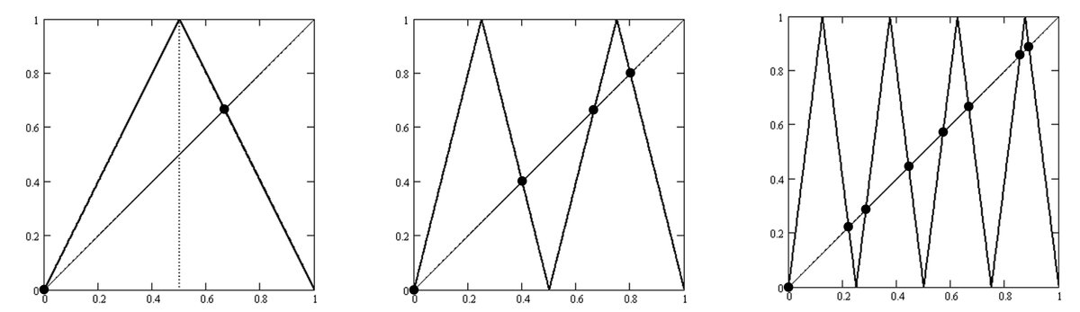
1-periodic points can be obtained from $${f(x)=x}$$. Therefore, from the x-coordinates of the two points in the left figure of Figure 5-4, $${0}$$and $${\cfrac{2}{3}}$$ are 1-periodic points, which are called fixed points.
The 2-periodic points can be obtained from the equation $${f^2(x)=f(f(x))=x}$$. Therefore, the x-coordinates of the four points in the middle figure of Figure 5-4 are candidates. Since the equation $${f^2(x)=f(f(x))=x}$$ also includes the solutions of $${f(x)=x}$$, the solutions are $${\cfrac{2}{5}}$$ and $${\cfrac{4}{5}}$$, excluding this.
The 3-periodic points can be obtained from the equation $${f^3(x)=f(f(f(x)))=x}$$. Therefore, the x-coordinates of the eight points in the right figure of Figure 5-4 are candidates. Since the equation $${f^3(x)=f(f(f(x)))=x}$$ also includes the two solutions of $${f(x)=x}$$, the
solutions are $${\cfrac{2}{9}}$$、$${\cfrac{2}{7}}$$、$${\cfrac{4}{9}}$$、$${\cfrac{4}{7}}$$、$${\cfrac{6}{7}}$$, and $${\cfrac{8}{9}}$$ excluding these two.
In general, the n-periodic points are the x-coordinates of all the intersection points of the n-th iterate of the map $${y=f^n(x)}$$ and $${y=x}$$ ($${2^n}$$ points in total) except for all the p-periodic points for all the divisors $${p}$$ of $${n}$$.
with y = x for 0 ≤ x < 1
Another example is the case of $${0 < a < 1}$$ in equation (5.1) with a=0.7. The left figure shows the cobweb diagram for the initial value 0.4, and the right figure shows the diagram for the initial value 0.7. The fixed point is $${x=0}$$. Regardless of the initial value $${x_0}$$ chosen between 0 and 1, the sequence converges to $${0}$$ as$${n}$$ approaches infinity.

Other famous one-dimensional maps include the Bernoulli shift (or binary shift) map and the logistic map. Both are important maps in chaos theory. You can find more information about them on other websites. The Bernoulli shift map is briefly introduced in Chapter 7 in relation to the Collatz conjecture.
I hope you have found the Lorenz plot and cobweb diagram to be useful tools.
Variables, Definitions, and Functions up to Chapter 5:
$${N}$$, $${No}$$,
total number of steps, step number, CS-vibration, C-transformation,
CS-plot, CS-linear-equations, 3C+1 transformation, 3S+1 transformation,
(general) Collatz space, CS-line, S-transformation, CS-space, t-tree,
Lorenz plot, period orbit, periodic point, eventually periodic point,
cobweb diagram, fixed point,
type $${6t+5}$$, $${6t+1}$$, $${4t+3}$$, $${8t+1}$$, etc.
$${c(No)}$$, $${z_{s}}$$, $${f_{c}(x)}$$, $${f_{s}(x)}$$, distance$${D}$$,
$${Nc}$$, $${Ns}$$, $${m_o}$$, $${m_{c}}$$, $${m_{s}}$$, $${t_{c}}$$, $${t_{s}}$$, $${t}$$, $${cs(m_o)}$$, $${Mo}$$, $${s(Mo)}$$,
change of pace: Monster Hunter
The content may have become a bit serious throughout each chapter,
but I assure you that I am not a rigid person.
Speaking of getting hooked, I was really hooked on the Monster Hunter series. I used to play Mario, The Legend of Zelda, Resident Evil, and Final Fantasy, and I enjoyed them all, but I haven't played anything but the Monster Hunter series since it came out.
The game requires swordsmanship skills and tactics, so it is a difficult game in that sense. Many people around me start playing because it's fun at first, but they stop playing halfway through because the difficulty of the monsters increases.
I don't feel like I've played the game unless it's on a big screen. I've played all of them on PlayStation, from the original Monster Hunter to Monster Hunter 2, ... I don't know what number it is, but I've played all of them up to Monster Hunter Iceborne (except for the ones that were only available online).
I timed out on the final boss of Yvelkhana in the Land of Crystals in Iceborne. Except for Alatreon, Fatalis, and, the final boss (meaning the strongest one) of Brachydios in the Volcanic Region (online-only monster from previous games), I've soloed all the other monsters, including those from other series. I've seen players on YouTube soloing monsters in seconds or minutes, but I'm not that skilled.
My main weapon is the Lance, which is a relatively unpopular choice. I also use the Greatsword and Dual Blades occasionally. I use the Bow, Hammer, Light and Heavy Bowguns depending on the monster. I used to use the Longsword, which is one of the most popular weapons, in the early series. I used the Insect Glaive for fun to fly around in the air against low-rank monsters. I only use the Charge Axe against Tigrex. I don't use the Switch Axe, Gunlance, or Sword and Shield very often, and I've never used the Hunting Horn.
There are many great songs in the soundtrack, including the theme song and each monster's appearance theme. Neko Village is also very cute.
I'm currently hooked on the Collatz conjecture (I got hooked on it),
so I haven't played since Iceborne. I might play it when the new game comes out, but I don't think I'll be as addicted as before.
Now that I have stumbled upon the world of unsolved mathematical problems, I feel differently.
・・・・・・・・・・・・・・・
この記事が気に入ったらサポートをしてみませんか?