TensorFlow 2.0 + Kerasの概要 / Part1: TensorFlowの基礎

「TensorFlow 2.0 + Keras Overview for Deep Learning Researchers」をベースに自分用に説明追加したものになります。

1. TensorFlow 2.0の準備

はじめに、「TensorFlow 2.0」をインストールします。

!pip install tensorflow==2.0.0

そして「tensorflow」をインポートします。

import tensorflow as tf
print(tf.__version__)

2.0.0

2. テンソル

定数テンソルを定義するには、次のように記述します。

x = tf.constant([[5, 2], [1, 3]])
print(x)

tf.Tensor(
[[5 2]
[1 3]], shape=(2, 2), dtype=int32)

numpy()を呼ぶことにより、その値をNumpy配列として取得することができます。

x.numpy()

array([[5, 2],
      [1, 3]], dtype=int32)

Numpy配列と同じように、「dtype」でデータ型、「shape」でシェイプを取得できます。

print('dtype:', x.dtype)
print('shape:', x.shape)

dtype: <dtype: 'int32'>
shape: (2, 2)

1埋めの定数テンソルはtf.ones()、0埋めの定数テンソルはtf.zeros()で作成します。np.ones()、np.zeros()と同様です。

print(tf.ones(shape=(2, 1)))
print(tf.zeros(shape=(2, 1)))

tf.Tensor(
[[1.]
[1.]], shape=(2, 1), dtype=float32)
tf.Tensor(
[[0.]
[0.]], shape=(2, 1), dtype=float32)

3. ランダムな定数テンソル

「正規分布」のランダムな定数テンソルはrandom.normal()で作成します。
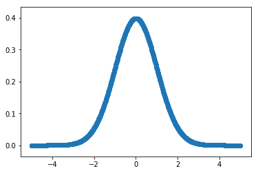
「正規分布」は名前の通りありふれている確率分布です。「平均値」(mean)と「中央値」が一致し、「標準偏差」(std)が大きくなると、曲線の山は低く、左右に広がって平らになります。

tf.random.normal(shape=(2, 2), mean=0., stddev=1.)

<tf.Tensor: id=12, shape=(2, 2), dtype=float32, numpy=
array([[ 0.4181472 , -0.26653227],
      [-0.50588334, -0.04563563]], dtype=float32)>

「一様分布」のランダムな定数テンソルはrandom.uniform()で作成します。
「一様分布」は、サイコロのそれぞれの目の出る確率など、すべての事象の起こる確率が等しい確率分布です。

tf.random.uniform(shape=(2, 2), minval=0, maxval=10, dtype='int32')

<tf.Tensor: id=20, shape=(2, 2), dtype=int32, numpy=
array([[2, 4],
      [3, 0]], dtype=int32)>

4. 変数

「Variable」は、ニューラルネットワークの重みなどの「変数」を保持するために使う特別なテンソルです。初期値を使用して作成します。

initial_value = tf.constant([1, 2])
a = tf.Variable(initial_value)
print(a)

<tf.Variable 'Variable:0' shape=(2,) dtype=int32, numpy=array([1, 2], dtype=int32)>

変数の値を変更するには、assign(value)を使用します。

new_value = tf.constant([1, 1])
a.assign(new_value)
print(a)

<tf.Variable 'Variable:0' shape=(2,) dtype=int32, numpy=array([1, 1], dtype=int32)>

変数の値を加算するには、assign_add(increment)を使用します。

add_value = tf.constant([1, 1])
a.assign_add(add_value)
print(a)

<tf.Variable 'Variable:0' shape=(2,) dtype=int32, numpy=array([2, 2], dtype=int32)>

変数の値を減算するには、assign_sub(decrement)を使用します。

del_value = tf.constant([1, 1])
a.assign_sub(del_value)
print(a)

<tf.Variable 'Variable:0' shape=(2,) dtype=int32, numpy=array([1, 1], dtype=int32)>

5. 数値演算

TensorFlowは、Numpyと同じように数値演算を使用できます。主な違いは、TensorFlowのコードは「GPU」と「TPU」で実行できることです。

a = tf.random.normal(shape=(2, 2))
b = tf.random.normal(shape=(2, 2))

c = a + b
d = tf.square(c)
e = tf.exp(d)

6. GradientTapeによる勾配計算

TensorFlowは、微分可能な式の勾配を自動計算できます。Numpyはできません。

「GradientTape」をオープンし、tape.watch()でテンソルの「監視」を開始し、このテンソルを入力とする微分可能な式を作成します。

a = tf.random.normal(shape=(2, 2))
b = tf.random.normal(shape=(2, 2))

with tf.GradientTape() as tape:
 tape.watch(a)  # aに適用された操作の履歴の記録を開始
 c = tf.sqrt(tf.square(a) + tf.square(b))  # aを使用して計算を行う
 dc_da = tape.gradient(c, a) # aに対するcの勾配を計算
 print(dc_da)

tf.Tensor(
[[-0.40515587  0.5971111 ]
[-0.8044381  -0.31810388]], shape=(2, 2), dtype=float32)

「変数」は自動的に監視されるため、手動で監視する必要はありません。

a = tf.Variable(a)

with tf.GradientTape() as tape:
 c = tf.sqrt(tf.square(a) + tf.square(b))
 dc_da = tape.gradient(c, a)
 print(dc_da)

tf.Tensor(
[[-0.40515587  0.5971111 ]
[-0.8044381  -0.31810388]], shape=(2, 2), dtype=float32)

テープをネストすることにより、高次の導関数を計算できます。

with tf.GradientTape() as outer_tape:
 with tf.GradientTape() as tape:
   c = tf.sqrt(tf.square(a) + tf.square(b))
   dc_da = tape.gradient(c, a)
 d2c_da2 = outer_tape.gradient(dc_da, a)
 print(d2c_da2)

7. 線形回帰の例

これまで「TensorFlow」は、「GPU」「TPU」で高速化され、勾配を自動計算できる、Numpyライクなライブラリであることを学びました。

次は例として、「線形回帰」を実装します。「回帰」は、複数の特徴データをもとに、連続値などの「数値」を予測するタスクです。「回帰」で使われる最も基本的なモデルは「線形回帰」と呼ばれ、目的変数「y」 と説明変数「xi」と重み「wi」とバイアス「b」を以下のようにモデル化したものになります。

デモンストレーションのために、 「Layer」や「MeanSquaredError」のような高レベルのKerasコンポーネントは使用しません。

input_dim = 2
output_dim = 1
learning_rate = 0.01

# 重み
w = tf.Variable(tf.random.uniform(shape=(input_dim, output_dim)))

# バイアス
b = tf.Variable(tf.zeros(shape=(output_dim,)))

# 予測の計算
def compute_predictions(features):
 return tf.matmul(features, w) + b

# 損失の計算
def compute_loss(labels, predictions):
 return tf.reduce_mean(tf.square(labels - predictions))

# 訓練
def train_on_batch(x, y):
 with tf.GradientTape() as tape:
   predictions = compute_predictions(x)
   loss = compute_loss(y, predictions)

   # tape.gradientはリスト[w, b]も適用可
   dloss_dw, dloss_db = tape.gradient(loss, [w, b])
 w.assign_sub(learning_rate * dloss_dw)
 b.assign_sub(learning_rate * dloss_db)
 return loss

モデルを示すために、いくつかのデータを生成します。

import numpy as np
import random
import matplotlib.pyplot as plt
%matplotlib inline

# データの準備
num_samples = 10000
negative_samples = np.random.multivariate_normal(
   mean=[0, 3], cov=[[1, 0.5],[0.5, 1]], size=num_samples)
positive_samples = np.random.multivariate_normal(
   mean=[3, 0], cov=[[1, 0.5],[0.5, 1]], size=num_samples)
features = np.vstack((negative_samples, positive_samples)).astype(np.float32)
labels = np.vstack((np.zeros((num_samples, 1), dtype='float32'), np.ones((num_samples, 1), dtype='float32')))

plt.scatter(features[:, 0], features[:, 1], c=labels[:, 0])

データをバッチごとに train_on_batch()を繰り返し呼び出して、「線形回帰」を学習します。

# データのシャッフル
indices = np.random.permutation(len(features))
features = features[indices]
labels = labels[indices]

# 簡単なバッチ反復のためにtf.data.Datasetオブジェクトを作成
dataset = tf.data.Dataset.from_tensor_slices((features, labels))
dataset = dataset.shuffle(buffer_size=1024).batch(256)

for epoch in range(10):
 for step, (x, y) in enumerate(dataset):
   loss = train_on_batch(x, y)
 print('Epoch %d: last batch loss = %.4f' % (epoch, float(loss)))

poch 0: last batch loss = 0.0631
Epoch 1: last batch loss = 0.0266
Epoch 2: last batch loss = 0.0318
Epoch 3: last batch loss = 0.0311
Epoch 4: last batch loss = 0.0326
Epoch 5: last batch loss = 0.0260
Epoch 6: last batch loss = 0.0131
Epoch 7: last batch loss = 0.0176
Epoch 8: last batch loss = 0.0325
Epoch 9: last batch loss = 0.0375

モデルのパフォーマンスは次の通りです。

predictions = compute_predictions(features)
plt.scatter(features[:, 0], features[:, 1], c=predictions[:, 0] > 0.5)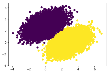

8. tf.functionによる高速化

現在のコードの実行速度を測定します。

import time

t0 = time.time()
for epoch in range(20):
 for step, (x, y) in enumerate(dataset):
   loss = train_on_batch(x, y)
t_end = time.time() - t0
print('Time per epoch: %.3f s' % (t_end / 20,))

Time per epoch: 0.200 s

ここで、訓練関数を「静的なグラフ」にコンパイルしてみます。「@tf.function」を追加するだけです。

@tf.function
def train_on_batch(x, y):
 with tf.GradientTape() as tape:
   predictions = compute_predictions(x)
   loss = compute_loss(y, predictions)
   dloss_dw, dloss_db = tape.gradient(loss, [w, b])
 w.assign_sub(learning_rate * dloss_dw)
 b.assign_sub(learning_rate * dloss_db)
 return loss

これをもう一度試してみます。

t0 = time.time()
for epoch in range(20):
 for step, (x, y) in enumerate(dataset):
   loss = train_on_batch(x, y)
t_end = time.time() - t0
print('Time per epoch: %.3f s' % (t_end / 20,))

Time per epoch: 0.104 s

40％削減されました。一般に、モデルが大きいほど、静的グラフを活用することで得られる速度向上が大きくなります。
Eagerな実行は、結果を行ごとにデバッグおよびprint()するのに最適ですが、速度に関しては「静的グラフ」が有効です。