Pythonで学ぶ技術者のための線形代数学と微分積分学

線形代数学
3次元ベクトルの外積
import numpy as np
import matplotlib.pyplot as plt
from mpl_toolkits.mplot3d import Axes3D

# 3次元ベクトルの定義
v1 = np.array([1, 2, 3])
v2 = np.array([4, 5, 6])

# 外積の計算
cross_product = np.cross(v1, v2)

# プロットのためのデータ準備
origin = np.zeros(3)
vectors = [origin, v1, origin, v2, origin, cross_product]

# 各ベクトルの始点と終点
X, Y, Z = zip(*vectors)

# プロット
fig = plt.figure()
ax = fig.add_subplot(111, projection='3d')
ax.quiver(X[::2], Y[::2], Z[::2], X[1::2], Y[1::2], Z[1::2], color=['r', 'b', 'g'], label=['v1', 'v2', 'cross_product'])
ax.scatter(X[::2], Y[::2], Z[::2], color=['r', 'b', 'g'])  # 始点をプロット
ax.scatter(X[1::2], Y[1::2], Z[1::2], color=['r', 'b', 'g'])  # 終点をプロット
ax.set_xlim([0, max(v1[0], v2[0], cross_product[0])])
ax.set_ylim([0, max(v1[1], v2[1], cross_product[1])])
ax.set_zlim([0, max(v1[2], v2[2], cross_product[2])])
ax.set_xlabel('X')
ax.set_ylabel('Y')
ax.set_zlabel('Z')
ax.set_title('3D Vector Plot')
plt.legend()
plt.show()
単位逆列
import numpy as np

# サイズが3x3の単位行列を作成
I = np.eye(3)

# 行列Aを作成(例として乱数を使用)
A = np.random.rand(3, 3)

# Aに単位行列を掛け算して、元の行列Aが得られることを確認
result = np.dot(A, I)

print("A:\n", A)
print("\nAに単位行列を掛けた結果:\n", result)
ゼロ行列
import numpy as np

# ゼロ行列のサイズを指定
rows = 3
cols = 4

# ゼロ行列の作成
zero_matrix = np.zeros((rows, cols))

print("ゼロ行列:\n", zero_matrix)
行列を逆行列にする
import numpy as np

# 元の行列の定義
matrix = np.array([[1, 2], [3, 4]])

# 行列の逆行列を計算
inverse_matrix = np.linalg.inv(matrix)

print("元の行列:\n", matrix)
print("\n逆行列:\n", inverse_matrix)
連立方程式を解く
import numpy as np

# 連立方程式の係数行列
A = np.array([[2, -1, 3],
              [1, 1, 1],
              [3, -2, 1]])

# 定数ベクトル
B = np.array([5, 3, 4])

# 行列式を計算
det_A = np.linalg.det(A)

# 行列式が0でない場合に解を計算
if det_A != 0:
    # 逆行列を使って解を計算
    X = np.linalg.inv(A).dot(B)
    print("解:", X)
else:
    print("行列式が0なので解は存在しません。")
平面の方程式
import numpy as np
import matplotlib.pyplot as plt
from mpl_toolkits.mplot3d import Axes3D

# 平面の方程式:ax + by + cz + d = 0
a, b, c, d = 1, 2, -3, 4

# 平面上の点
point_on_plane = np.array([1, 2, 3])

# 観測点
observed_point = np.array([4, 5, 6])

# 平面と観測点の距離を求める
distance = np.abs(np.dot(np.array([a, b, c]), observed_point) + d) / np.linalg.norm(np.array([a, b, c]))

print("Distance between the point and the plane:", distance)

# 平面の方程式をプロット
fig = plt.figure()
ax = fig.add_subplot(111, projection='3d')

# 平面の方程式
x = np.linspace(-10, 10, 100)
y = np.linspace(-10, 10, 100)
X, Y = np.meshgrid(x, y)
Z = (-a * X - b * Y - d) / c

ax.plot_surface(X, Y, Z, alpha=0.5)

# 点をプロット
ax.scatter(point_on_plane[0], point_on_plane[1], point_on_plane[2], color='red', label='Point on Plane')
ax.scatter(observed_point[0], observed_point[1], observed_point[2], color='blue', label='Observed Point')

ax.set_xlabel('X')
ax.set_ylabel('Y')
ax.set_zlabel('Z')
ax.legend()

plt.show()
ヴァンデルモンドの行列式と巡回行列式
import numpy as np

def vandermonde_det(A):
    """
    ヴァンデルモンドの行列式を計算する関数
    :param A: 入力の行列 (numpy array)
    :return: 行列式の値
    """
    n = A.shape[0]
    if n != A.shape[1]:
        raise ValueError("Input matrix must be square")
    return np.prod([A[i, j] - A[i, k] for i in range(n) for j in range(i+1, n) for k in range(i)])

def circulant_det(A):
    """
    巡回行列式を計算する関数
    :param A: 入力の行列 (numpy array)
    :return: 行列式の値
    """
    n = A.shape[0]
    if n != A.shape[1]:
        raise ValueError("Input matrix must be square")
    return np.prod([np.sum(np.linalg.eigvals(A)**k) for k in range(n)])

# 例として、3x3のヴァンデルモンド行列と巡回行列の行列式を計算します
vandermonde_matrix = np.array([[1, 2, 3],
                               [1, 4, 9],
                               [1, 8, 27]])

circulant_matrix = np.array([[1, 2, 3],
                             [3, 1, 2],
                             [2, 3, 1]])

print("Vandermonde determinant:", vandermonde_det(vandermonde_matrix))
print("Circulant determinant:", circulant_det(circulant_matrix))
対角化
import numpy as np
import matplotlib.pyplot as plt

# 3x3行列の設定
A = np.array([[1, 2, 3],
              [4, 5, 6],
              [7, 8, 9]])

# 固有値と固有ベクトルの計算
eigenvalues, eigenvectors = np.linalg.eig(A)

# 正則行列の作成
regular_matrix = np.array([[2, 3, 4],
                           [5, 6, 7],
                           [8, 9, 10]])

# 正則行列の対角化
diagonal_matrix = np.diag(np.diag(regular_matrix))

# 結果の表示
print("行列Aの固有値:", eigenvalues)
print("行列Aの固有ベクトル:\n", eigenvectors)
print("正則行列の対角行列:\n", diagonal_matrix)

# プロット
plt.figure()

# 固有値のプロット
plt.subplot(1, 3, 1)
plt.plot(eigenvalues, 'ro')
plt.title('Eigenvalues')

# 固有ベクトルのプロット
plt.subplot(1, 3, 2)
for i in range(len(eigenvectors)):
    plt.plot(eigenvectors[:, i], label='Eigenvec {}'.format(i+1))
plt.title('Eigenvectors')
plt.legend()

# 対角行列のプロット
plt.subplot(1, 3, 3)
plt.imshow(diagonal_matrix, cmap='viridis')
plt.colorbar()
plt.title('Diagonal Matrix')

plt.tight_layout()
plt.show()
アダマール積 行列
import numpy as np

# 2つの行列を生成
A = np.array([[1, 2, 3],
              [4, 5, 6]])

B = np.array([[7, 8, 9],
              [10, 11, 12]])

# アダマール積を計算
Hadamard_product = A * B

print("A:\n", A)
print("B:\n", B)
print("Hadamard product (A ⊙ B):\n", Hadamard_product)
ジョルダン標準形
import numpy as np

# システムの状態空間表現を定義する
A = np.array([[2, 1, 0],
              [0, 2, 0],
              [0, 0, 3]])

B = np.array([[1],
              [0],
              [0]])

C = np.array([[1, 0, 0]])

D = np.array([[0]])

# システムの状態空間表現を連結する
ss_system = np.vstack([
    np.hstack([A, B]),
    np.hstack([C, D])
])

# システムのジョルダン標準形を計算する
eigenvalues, P = np.linalg.eig(A)
n = len(A)
Jordan_blocks = []

for eigenvalue in eigenvalues:
    block_size = np.sum(np.abs(eigenvalues - eigenvalue) < 1e-9)  # ほぼ等しい固有値の数を数える
    jordan_block = eigenvalue * np.eye(block_size) + np.diag(np.ones(block_size - 1), 1)
    Jordan_blocks.append(jordan_block)

Jordan_block_diag = np.block(Jordan_blocks)

# 状態空間表現に変換行列を適用する
P_inv = np.linalg.inv(P)
Jordan_standard_form = P_inv @ Jordan_block_diag @ P

# ジョルダン標準形を表示する
print("Jordan Canonical Form:")
print(Jordan_standard_form)
言葉のベクトル化
from gensim.models import Word2Vec
import matplotlib.pyplot as plt

# サンプルの文書データ
sentences = [["I", "love", "natural", "language", "processing"],
             ["Word", "embeddings", "are", "useful"],
             ["Natural", "language", "processing", "is", "challenging"]]

# Word2Vecモデルの学習
model = Word2Vec(sentences, vector_size=2, window=5, min_count=1, sg=1)

# 単語のベクトルをプロット
for word in model.wv.index_to_key:
    plt.annotate(word, xy=model.wv[word])
    plt.scatter(model.wv[word][0], model.wv[word][1])

plt.xlabel('Dimension 1')
plt.ylabel('Dimension 2')
plt.title('Word Vectors')

plt.show()
微分積分学
グラフの描写
import numpy as np
import matplotlib.pyplot as plt

# グラフの範囲
x = np.linspace(-2*np.pi, 2*np.pi, 1000)

# 三角関数
sinx = np.sin(x)
cosx = np.cos(x)
tanx = np.tan(x)

# 逆三角関数
arcsinx = np.arcsin(x)
arccosx = np.arccos(x)
arctanx = np.arctan(x)

# 双曲線関数
sinhx = np.sinh(x)
coshx = np.cosh(x)
tanhx = np.tanh(x)

# 逆双曲線関数
arcsinhx = np.arcsinh(x)
arccoshx = np.arccosh(x)
arctanhx = np.arctanh(x)

# グラフの描画
plt.figure(figsize=(12, 8))

# 三角関数のプロット
plt.subplot(3, 4, 1)
plt.plot(x, sinx, label='sin(x)')
plt.legend()

plt.subplot(3, 4, 2)
plt.plot(x, cosx, label='cos(x)')
plt.legend()

plt.subplot(3, 4, 3)
plt.plot(x, tanx, label='tan(x)')
plt.ylim(-5, 5)  # tan(x)の範囲を調整
plt.legend()

# 逆三角関数のプロット
plt.subplot(3, 4, 4)
plt.plot(x, arcsinx, label='arcsin(x)')
plt.legend()

plt.subplot(3, 4, 5)
plt.plot(x, arccosx, label='arccos(x)')
plt.legend()

plt.subplot(3, 4, 6)
plt.plot(x, arctanx, label='arctan(x)')
plt.legend()

# 双曲線関数のプロット
plt.subplot(3, 4, 7)
plt.plot(x, sinhx, label='sinh(x)')
plt.legend()

plt.subplot(3, 4, 8)
plt.plot(x, coshx, label='cosh(x)')
plt.legend()

plt.subplot(3, 4, 9)
plt.plot(x, tanhx, label='tanh(x)')
plt.ylim(-2, 2)  # tanh(x)の範囲を調整
plt.legend()

# 逆双曲線関数のプロット
plt.subplot(3, 4, 10)
plt.plot(x, arcsinhx, label='arcsinh(x)')
plt.legend()

plt.subplot(3, 4, 11)
plt.plot(x, arccoshx, label='arccosh(x)')
plt.ylim(0, 4)  # arccosh(x)の範囲を調整
plt.legend()

plt.subplot(3, 4, 12)
plt.plot(x, arctanhx, label='arctanh(x)')
plt.ylim(-2, 2)  # arctanh(x)の範囲を調整
plt.legend()

plt.tight_layout()
plt.show()
三相交流
import numpy as np
import matplotlib.pyplot as plt

# 時間軸の定義
t = np.linspace(0, 2*np.pi, 1000)  # 0から2πまでの1000点の時間軸

# 三相交流波形の定義
phase_shift = 2*np.pi/3  # 位相差
amplitude = 1  # 振幅

# 三相交流波形
phase_1 = amplitude * np.sin(t)
phase_2 = amplitude * np.sin(t - phase_shift)
phase_3 = amplitude * np.sin(t - 2*phase_shift)

# プロット
plt.plot(t, phase_1, label='Phase 1')
plt.plot(t, phase_2, label='Phase 2')
plt.plot(t, phase_3, label='Phase 3')
plt.title('Three Phase AC Waveforms')
plt.xlabel('Time (t)')
plt.ylabel('Amplitude')
plt.legend()
plt.grid(True)
plt.show()
増幅率の計算
import numpy as np
import matplotlib.pyplot as plt

# パラメータ設定
# Aは増幅 R1とR2は抵抗
A = 10000
R1 = 10
R2 = 20
f = 1  # サイン波の周波数
t = np.linspace(0, 1, 1000)  # 時間配列

# 反転増幅率の計算
inverting_gain = -R2 / (((R1 + R2) / A) + R1)

# 非反転増幅率の計算
noninverting_gain = 1 / ((1 / A) + ((R1 + R2) / R2))

print("反転増幅率:", inverting_gain)
print("非反転増幅率:", noninverting_gain)

# 入力信号(サイン波)
input_signal = np.sin(2 * np.pi * f * t)

# 反転増幅器出力
inverting_amplifier_output = (-R2 / (((R1 + R2) / A) + R1)) * input_signal

# 非反転増幅器出力
noninverting_amplifier_output = (1 / ((1 / A) + ((R1 + R2) / R2))) * input_signal

# 反転増幅率と非反転増幅率の時間による変化をプロット
plt.figure(figsize=(10, 6))

plt.plot(t, inverting_gain * np.ones_like(t), label='Inverting Gain', linestyle='--')
plt.plot(t, noninverting_gain * np.ones_like(t), label='Noninverting Gain', linestyle='--')

plt.title('Inverting and Noninverting Gain vs. Time')
plt.xlabel('Time')
plt.ylabel('Gain')
plt.legend()

plt.tight_layout()
plt.show()

# プロット
plt.figure(figsize=(10, 6))

plt.subplot(2, 1, 1)
plt.plot(t, inverting_amplifier_output, label='Inverting Amplifier Output')
plt.plot(t, input_signal, label='Input Signal')
plt.title('Inverting Amplifier Output vs. Input Signal')
plt.xlabel('Time')
plt.ylabel('Amplitude')
plt.legend()

plt.subplot(2, 1, 2)
plt.plot(t, noninverting_amplifier_output, label='Noninverting Amplifier Output')
plt.plot(t, input_signal, label='Input Signal')
plt.title('Noninverting Amplifier Output vs. Input Signal')
plt.xlabel('Time')
plt.ylabel('Amplitude')
plt.legend()

plt.tight_layout()
plt.show()
差動増幅
import numpy as np
import matplotlib.pyplot as plt

# 時間軸の作成
t = np.linspace(0, 2*np.pi, 1000)

# プラス入力(t)とマイナス入力(t)の計算
plus_input = np.sin(t)
minus_input = np.cos(t)

# 出力波形の計算
amplification = 30
output = amplification * (plus_input - minus_input)

# プラス入力とマイナス入力のプロット
plt.figure(figsize=(10, 6))
plt.plot(t, plus_input, label='プラス入力')
plt.plot(t, minus_input, label='マイナス入力')
plt.title('プラス入力とマイナス入力の時間変化')
plt.xlabel('時間')
plt.ylabel('値')
plt.legend()
plt.grid(True)
plt.show()

# 出力波形のプロット
plt.figure(figsize=(10, 6))
plt.plot(t, output, label='出力')
plt.title('出力の時間変化')
plt.xlabel('時間')
plt.ylabel('値')
plt.legend()
plt.grid(True)
plt.show()
オイラーの公式
import numpy as np
import matplotlib.pyplot as plt

# 角度(ラジアン)を設定
angle = 0.16 * np.pi

# オイラーの公式に角度を代入して複素数を計算
complex_number = np.exp(1j * angle)

# プロット
plt.figure(figsize=(8, 8))
plt.plot(np.real(complex_number), np.imag(complex_number), 'ro')
plt.axhline(0, color='black',linewidth=0.5)
plt.axvline(0, color='black',linewidth=0.5)
plt.grid(color = 'gray', linestyle = '--', linewidth = 0.5)
plt.xlabel('Real')
plt.ylabel('Imaginary')
plt.title('Complex Number Plot with Euler\'s Formula')
plt.gca().set_aspect('equal', adjustable='box')
plt.show()
import sympy as sp
import numpy as np
import matplotlib.pyplot as plt

# シンボルの定義
t, a, n = sp.symbols('t a n')

# aとnの値の定義
a_val = 1
n_val = 0

# 関数の定義
f = sp.sin(a*t + n)

# 微分
df_dt = sp.diff(f, t)

# 積分
integral_f = sp.integrate(f, t)

# tの値の範囲を定義
t_values = np.linspace(-10, 10, 1000)

# 関数の値を計算
f_values = np.array([f.subs({t: val, a: a_val, n: n_val}).evalf() for val in t_values])
df_dt_values = np.array([df_dt.subs({t: val, a: a_val, n: n_val}).evalf() for val in t_values])
integral_f_values = np.array([integral_f.subs({t: val, a: a_val, n: n_val}).evalf() for val in t_values])

# グラフのプロット
plt.figure(figsize=(10, 6))

# 元の関数のプロット
plt.subplot(3, 1, 1)
plt.plot(t_values, f_values, label='sin(at+n)')
plt.xlabel('t')
plt.ylabel('f(t)')
plt.title('Original Function')
plt.grid()
plt.legend()

# 微分した関数のプロット
plt.subplot(3, 1, 2)
plt.plot(t_values, df_dt_values, label="df/dt")
plt.xlabel('t')
plt.ylabel("df(t)/dt")
plt.title('Derivative')
plt.grid()
plt.legend()

# 積分した関数のプロット
plt.subplot(3, 1, 3)
plt.plot(t_values, integral_f_values, label="integral of f(t)")
plt.xlabel('t')
plt.ylabel("Integral of f(t)")
plt.title('Integral')
plt.grid()
plt.legend()

plt.tight_layout()
plt.show()
トランジスタの線形領域と飽和領域
import numpy as np
import matplotlib.pyplot as plt

# 定数定義
VDD = 5.0  # V
VGS = 2.0  # V
VTH = 1.0  # V
Rd = 1e3   # ソース抵抗, 1kΩ
K = 0.5e-3 # トランジスタの係数, 0.5mA/V^2

# VDSの範囲を定義
VDS_range = np.linspace(0, VDD, 100)

# VDSに対するIDSの関数を定義
def calculate_IDS(VDS):
    if VGS <= VTH:
        return 0
    elif VDS < VGS - VTH:
        return K * (2 * (VGS - VTH) * VDS - VDS**2) / 2
    else:
        return K * (VGS - VTH)**2 / 2

# VDSに対するIDSを計算
IDS_values = [calculate_IDS(VDS) for VDS in VDS_range]

# グラフの描画
plt.plot(VDS_range, IDS_values, label='IDS')
plt.xlabel('VDS (V)')
plt.ylabel('IDS (A)')
plt.title('Transistor Characteristics')
plt.grid(True)
plt.legend()
plt.show()
ラグランジュの未定乗数法
import numpy as np
import matplotlib.pyplot as plt

# 目的関数の定義
def objective(x):
    return x[0]**2 + x[1]**2

# 制約条件関数の定義
def constraint(x):
    return x[0] + x[1] - 1

# 等高線プロットのための範囲定義
x_values = np.linspace(-1, 2, 400)
y_values = np.linspace(-1, 2, 400)
X, Y = np.meshgrid(x_values, y_values)
Z = X**2 + Y**2

# 制約条件をプロット
plt.contour(X, Y, Z, levels=20, cmap='RdBu')
plt.colorbar(label='f(x, y)')
plt.contour(X, Y, X + Y - 1, levels=[0], colors='red', linestyles='dashed', linewidths=2)
plt.xlabel('x')
plt.ylabel('y')
plt.title('Contour Plot with Constraint')
plt.grid(True)
plt.show()
import numpy as np
import matplotlib.pyplot as plt
from mpl_toolkits.mplot3d import Axes3D

# 関数の定義
def f(x, y):
    return x**2 + y**2

# x, yの値の範囲
x_values = np.linspace(-2, 2, 100)
y_values = np.linspace(-2, 2, 100)
X, Y = np.meshgrid(x_values, y_values)

# 関数値の計算
Z = f(X, Y)

# プロット
fig = plt.figure(figsize=(8, 6))
ax = fig.add_subplot(111, projection='3d')
ax.plot_surface(X, Y, Z, cmap='viridis')
ax.set_xlabel('X')
ax.set_ylabel('Y')
ax.set_zlabel('f(X, Y)')
ax.set_title('Surface Plot of f(X, Y)')

# 最大値と最小値の計算
max_value = np.max(Z)
min_value = np.min(Z)
max_pos = np.unravel_index(np.argmax(Z), Z.shape)
min_pos = np.unravel_index(np.argmin(Z), Z.shape)
max_x, max_y = x_values[max_pos[1]], y_values[max_pos[0]]
min_x, min_y = x_values[min_pos[1]], y_values[min_pos[0]]

# 結果の出力
print("最大値:", max_value, "座標:", (max_x, max_y))
print("最小値:", min_value, "座標:", (min_x, min_y))

plt.show()
機械学習、制御工学、信号処理で使用する関数
import numpy as np
import matplotlib.pyplot as plt
from scipy.stats import norm

# サンプルデータの生成
x = np.linspace(-5, 5, 1000)

# 単位ステップ関数
step_function = np.heaviside(x, 1)

# ランプ波
ramp_wave = np.maximum(0, x)

# シグモイド関数
sigmoid_function = 1 / (1 + np.exp(-x))

# 単位インパルス関数(ディラックのデルタ関数の離散版)
impulse_function = np.zeros_like(x)
impulse_function[len(x)//2] = 1

# 正規分布の確率密度関数
pdf_normal_distribution = norm.pdf(x, loc=0, scale=1)

# プロット
plt.figure(figsize=(12, 8))

plt.subplot(3, 2, 1)
plt.plot(x, step_function, label='Unit Step Function')
plt.xlabel('x')
plt.ylabel('y')
plt.title('Unit Step Function')
plt.legend()

plt.subplot(3, 2, 2)
plt.plot(x, ramp_wave, label='Ramp Wave')
plt.xlabel('x')
plt.ylabel('y')
plt.title('Ramp Wave')
plt.legend()

plt.subplot(3, 2, 3)
plt.plot(x, sigmoid_function, label='Sigmoid Function')
plt.xlabel('x')
plt.ylabel('y')
plt.title('Sigmoid Function')
plt.legend()

plt.subplot(3, 2, 4)
plt.stem(x, impulse_function, label='Unit Impulse Function', use_line_collection=True)
plt.xlabel('x')
plt.ylabel('y')
plt.title('Unit Impulse Function')
plt.legend()

plt.subplot(3, 2, 5)
plt.plot(x, pdf_normal_distribution, label='Normal Distribution PDF')
plt.xlabel('x')
plt.ylabel('Probability Density')
plt.title('Normal Distribution PDF')
plt.legend()

plt.tight_layout()
plt.show()
サンプリング定理
import numpy as np
import matplotlib.pyplot as plt

# 入力波形の定義
t = np.linspace(0, 20, 1000)
input_waveform = np.sin(t)

# クロック波の定義
T = 1  # 周期
clock_waveform = np.zeros_like(t)
for i in range(len(t)):
    if t[i] % T < T/2:
        clock_waveform[i] = 1

# (nT, sin(nT))の点の定義
n_values = np.arange(1, 21)  # 自然数 1から20まで
x_points = n_values * T
y_points = np.sin(x_points)

# プロット
plt.figure(figsize=(12, 8))

# 入力波形のプロット
plt.subplot(3, 1, 1)
plt.plot(t, input_waveform, label='Input Waveform (sin(t))')
plt.xlabel('t')
plt.ylabel('Amplitude')
plt.title('Input Waveform')
plt.legend()

# クロック波のプロット
plt.subplot(3, 1, 2)
plt.plot(t, clock_waveform, label='Clock Waveform')
plt.xlabel('t')
plt.ylabel('Amplitude')
plt.title('Clock Waveform')
plt.legend()

# (nT, sin(nT))のプロット
plt.subplot(3, 1, 3)
plt.plot(x_points, y_points, 'ro', label='(nT, sin(nT)) Points')
plt.xlabel('t')
plt.ylabel('Amplitude')
plt.title('(nT, sin(nT)) Points')
plt.xticks(np.arange(0, 21, 1))  # x軸の目盛りを整数に設定
plt.legend()

plt.tight_layout()
plt.show()
import numpy as np
import matplotlib.pyplot as plt

# パラメータの設定
#2^nビットは2^n-1レベル


n = 4  # ビット数
FS = 10  # FSの値(仮の値)

# レベルの計算 Lは1LSB
L = FS / (2**n - 1)

# 関数の定義
def f(t):
    return L * np.sin(t) + L

# グラフのプロット
t_values = np.linspace(0, 2*np.pi, 1000)  # 0から2πまでのtの値を生成
f_values = f(t_values)  # 対応するf(t)の値を計算

plt.plot(t_values, f_values, label='f(t)=L*sin(t)+L')

# Tとf(T)をプロット
T = np.pi / 2  # 例えばTをπ/2とする
plt.plot(T, f(T), 'ro', label=f'(T, f(T)) = ({T:.2f}, {f(T):.2f})')
plt.plot(T, f(0), 'go', label=f'(T, f(0)) = ({T:.2f}, {f(0):.2f})')

plt.xlabel('t')
plt.ylabel('f(t)')
plt.title('f(t) = L*sin(t) + L')
plt.legend()
plt.grid(True)
plt.show()
A = 53

# Aのビット数を計算して表示
bit_count = A.bit_length()
print("Aのビット数:", bit_count)

# Aを2進数にして表示
binary_A = bin(A)
print("Aの2進数表現:", binary_A)

# 2進数にしたAとMSBとLSBを表示
MSB = binary_A[2]
LSB = binary_A[-1]
print("Aの2進数表現:", binary_A[2:], ", MSB:", MSB, ", LSB:", LSB)

# 2進数のAの2の補数表現を表示
two_complement = bin(A & 0b11111111)[-bit_count:]
print("Aの2の補数表現:", two_complement)
import numpy as np
import matplotlib.pyplot as plt

# サンプリング周波数
fs = 8192
# 信号の時間軸
t = np.arange(0, 1, 1/fs)

# 信号の生成
f_t = 0.3 * np.sin(2 * np.pi * 1000 * t) + \
      0.4 * np.sin(2 * np.pi * 2000 * t) + \
      0.2 * np.sin(2 * np.pi * 3000 * t)

# FFTを計算
fft_result = np.fft.fft(f_t)
# 振幅スペクトルを計算
magnitude_spectrum = np.abs(fft_result)
# 周波数軸を作成
freqs = np.fft.fftfreq(len(f_t), 1/fs)

# グラフ描画
plt.figure(figsize=(10, 6))

# 時間領域の信号のプロット
plt.subplot(2, 1, 1)
plt.plot(t, f_t)
plt.title('Signal in Time Domain')
plt.xlabel('Time [s]')
plt.ylabel('Amplitude')

# 振幅スペクトルのプロット
plt.subplot(2, 1, 2)
plt.plot(freqs[:len(freqs)//2], magnitude_spectrum[:len(freqs)//2])
plt.title('Magnitude Spectrum')
plt.xlabel('Frequency [Hz]')
plt.ylabel('Magnitude')

plt.tight_layout()
plt.show()
FFT
import numpy as np
import matplotlib.pyplot as plt

# サンプリング周波数
fs = 8192
# 信号の時間軸
t = np.arange(0, 1, 1/fs)

# 信号の生成
f_t = 0.3 * np.sin(2 * np.pi * 1000 * t) + \
      0.4 * np.sin(2 * np.pi * 2000 * t) + \
      0.2 * np.sin(2 * np.pi * 3000 * t)

# FFTを計算
fft_result = np.fft.fft(f_t)
# 振幅スペクトルを計算
magnitude_spectrum = np.abs(fft_result)
# パワースペクトルを計算
power_spectrum = np.abs(fft_result)**2 / len(f_t)
# 周波数軸を作成
freqs = np.fft.fftfreq(len(f_t), 1/fs)

# 振幅スペクトルから逆FFTを計算して波形を復元
reconstructed_signal = np.fft.ifft(fft_result)

# グラフ描画
plt.figure(figsize=(12, 10))

# 時間領域の信号と復元された信号のプロット
plt.subplot(4, 1, 1)
plt.plot(t, f_t, label='Original Signal', alpha=0.7)
plt.plot(t, reconstructed_signal, label='Reconstructed Signal', linestyle='--')
plt.title('Original vs Reconstructed Signal')
plt.xlabel('Time [s]')
plt.ylabel('Amplitude')
plt.legend()

# 振幅スペクトルのプロット
plt.subplot(4, 1, 2)
plt.plot(freqs[:len(freqs)//2], magnitude_spectrum[:len(freqs)//2])
plt.title('Magnitude Spectrum')
plt.xlabel('Frequency [Hz]')
plt.ylabel('Magnitude')

# パワースペクトルのプロット
plt.subplot(4, 1, 3)
plt.plot(freqs[:len(freqs)//2], power_spectrum[:len(freqs)//2])
plt.title('Power Spectrum')
plt.xlabel('Frequency [Hz]')
plt.ylabel('Power')

# 元の信号のプロット
plt.subplot(4, 1, 4)
plt.plot(t, f_t)
plt.title('Signal in Time Domain')
plt.xlabel('Time [s]')
plt.ylabel('Amplitude')

plt.tight_layout()
plt.show()
加法定理3Dプロット
import numpy as np
import matplotlib.pyplot as plt
from mpl_toolkits.mplot3d import Axes3D

# グリッドの作成
x = np.linspace(-2*np.pi, 2*np.pi, 100)
y = np.linspace(-2*np.pi, 2*np.pi, 100)
x, y = np.meshgrid(x, y)

# sin(x+y)とcos(x+y)の計算
z1 = np.sin(x + y)
z2 = np.cos(x + y)

# 最大値と最小値の計算
max_value = max(np.max(z1), np.max(z2))
min_value = min(np.min(z1), np.min(z2))

# 3Dプロット
fig = plt.figure()
ax = fig.add_subplot(111, projection='3d')

# sin(x+y)
ax.plot_surface(x, y, z1, cmap='viridis', alpha=0.7)
# cos(x+y)
ax.plot_surface(x, y, z2, cmap='plasma', alpha=0.7)

# 最大値と最小値をプロット
ax.scatter(0, 0, max_value, color='red', label=f'Max Value: {max_value:.2f}')
ax.scatter(0, 0, min_value, color='blue', label=f'Min Value: {min_value:.2f}')

# ラベルと凡例
ax.set_xlabel('X')
ax.set_ylabel('Y')
ax.set_zlabel('Z')
ax.legend()

plt.show()
テイラー展開 工学では誤差1%でもよい
import numpy as np
import matplotlib.pyplot as plt

# (1+x)^n のテイラー展開
def taylor_expansion_1plusx(x, n):
    result = 0
    for i in range(n + 1):
        result += np.math.comb(n, i) * (x ** i)
    return result

# e^x のテイラー展開
def taylor_expansion_ex(x, n):
    result = 0
    for i in range(n + 1):
        result += (x ** i) / np.math.factorial(i)
    return result

# sin(x) のテイラー展開
def taylor_expansion_sin(x, n):
    result = 0
    for i in range(n + 1):
        result += ((-1) ** i) * (x ** (2 * i + 1)) / np.math.factorial(2 * i + 1)
    return result

# cos(x) のテイラー展開
def taylor_expansion_cos(x, n):
    result = 0
    for i in range(n + 1):
        result += ((-1) ** i) * (x ** (2 * i)) / np.math.factorial(2 * i)
    return result

# (1/(1-x)) のテイラー展開
def taylor_expansion_1over1minusx(x, n):
    result = 0
    for i in range(n + 1):
        result += x ** i
    return result

# (1/(1+x)) のテイラー展開
def taylor_expansion_1over1plusx(x, n):
    result = 0
    for i in range(n + 1):
        result += (-1) ** i * x ** i
    return result

# プロットする範囲
x_values = np.linspace(-2, 2, 400)

# 各関数のテイラー展開を計算
n = 5
y_1plusx = [taylor_expansion_1plusx(x, n) for x in x_values]
y_ex = [taylor_expansion_ex(x, n) for x in x_values]
y_sin = [taylor_expansion_sin(x, n) for x in x_values]
y_cos = [taylor_expansion_cos(x, n) for x in x_values]
y_1over1minusx = [taylor_expansion_1over1minusx(x, n) for x in x_values]
y_1over1plusx = [taylor_expansion_1over1plusx(x, n) for x in x_values]

# プロット
plt.figure(figsize=(10, 6))

plt.subplot(231)
plt.plot(x_values, y_1plusx)
plt.title('(1+x)^n')

plt.subplot(232)
plt.plot(x_values, y_ex)
plt.title('e^x')

plt.subplot(233)
plt.plot(x_values, y_sin)
plt.title('sin(x)')

plt.subplot(234)
plt.plot(x_values, y_cos)
plt.title('cos(x)')

plt.subplot(235)
plt.plot(x_values, y_1over1minusx)
plt.title('1/(1-x)')

plt.subplot(236)
plt.plot(x_values, y_1over1plusx)
plt.title('1/(1+x)')

plt.tight_layout()
plt.show()
三角関数とテイラー展開線形近似の誤差を確認
import matplotlib.pyplot as plt
import numpy as np

# 関数A(n)
def A(n):
    return abs((np.sin(n*np.pi/180) - n*np.pi/180) * (180/np.pi))

# 関数B(n)
def B(n):
    return abs((np.cos(n*np.pi/180) - 1) * (180/np.pi))

# 点の数
num_points = 90

# nの値を生成
n_values = np.linspace(1, num_points, num_points)

# A(n)とB(n)の値を計算
A_values = [A(n) for n in n_values]
B_values = [B(n) for n in n_values]

# プロット
plt.plot(n_values, A_values, 'bo', label='A(n)')  # 青い点でプロット
plt.plot(n_values, B_values, 'ro', label='B(n)')  # 赤い点でプロット
plt.xlabel('n')
plt.ylabel('Value')
plt.title('Plot of A(n) and B(n)')
plt.legend()
plt.grid(True)
plt.show()

# 点を羅列
print("A(n)の点:")
for n, value in zip(n_values, A_values):
    print(f"n = {n}, A(n) = {value}")

print("\nB(n)の点:")
for n, value in zip(n_values, B_values):
    print(f"n = {n}, B(n) = {value}")
逆ラプラス変換と伝達関数
import numpy as np
import matplotlib.pyplot as plt
from scipy import signal

# 伝達関数の係数
a = 1
b = 2
c = 1

# 伝達関数の分子と分母の係数
numerator = [1]
denominator = [a, b, c]

# 逆ラプラス変換による解法
t, y = signal.impulse(signal.TransferFunction(numerator, denominator))

# 時間応答のプロット
plt.figure()
plt.plot(t, y)
plt.xlabel('Time')
plt.ylabel('Response')
plt.title('Inverse Laplace Transform')
plt.grid(True)
plt.show()

# ボード線図のプロット
w, mag, phase = signal.bode(signal.TransferFunction(numerator, denominator))
plt.figure()
plt.semilogx(w, mag)
plt.xlabel('Frequency [rad/s]')
plt.ylabel('Magnitude [dB]')
plt.title('Bode Plot')
plt.grid(True)
plt.show()

# ナイキスト線図のプロット
w, h = signal.freqresp(signal.TransferFunction(numerator, denominator))
plt.figure()
plt.plot(h.real, h.imag)
plt.xlabel('Real')
plt.ylabel('Imaginary')
plt.title('Nyquist Plot')
plt.grid(True)
plt.show()
波
import numpy as np
import matplotlib.pyplot as plt

# 方形波の生成
def square_wave(x, period):
    return np.sign(np.sin(2 * np.pi * x / period))

# 三角波の生成
def triangle_wave(x, period):
    return np.abs((2 * x / period - 1) % 2 - 1) * 2 - 1

# のこぎり波の生成
def sawtooth_wave(x, period):
    return 2 * (x / period - np.floor(0.5 + x / period))

# パルス波の生成
def pulse_wave(x, period, duty_cycle):
    return np.where((x % period) < period * duty_cycle, 1, -1)

# プロットする範囲
x_values = np.linspace(0, 4, 1000)

# 波形のパラメータ
period = 1.0  # 周期
duty_cycle = 0.5  # パルス波のデューティサイクル

# 波形の計算
square = square_wave(x_values, period)
triangle = triangle_wave(x_values, period)
sawtooth = sawtooth_wave(x_values, period)
pulse = pulse_wave(x_values, period, duty_cycle)

# プロット
plt.figure(figsize=(10, 6))

plt.subplot(221)
plt.plot(x_values, square)
plt.title('Square Wave')

plt.subplot(222)
plt.plot(x_values, triangle)
plt.title('Triangle Wave')

plt.subplot(223)
plt.plot(x_values, sawtooth)
plt.title('Sawtooth Wave')

plt.subplot(224)
plt.plot(x_values, pulse)
plt.title('Pulse Wave')

plt.tight_layout()
plt.show()
波形のフーリエ変換
import numpy as np
import matplotlib.pyplot as plt

# 波形の生成
def square_wave(x, period):
    return np.sign(np.sin(2 * np.pi * x / period))

def triangle_wave(x, period):
    return np.abs((2 * x / period - 1) % 2 - 1) * 2 - 1

def sawtooth_wave(x, period):
    return 2 * (x / period - np.floor(0.5 + x / period))

def pulse_wave(x, period, duty_cycle):
    return np.where((x % period) < period * duty_cycle, 1, -1)

# フーリエ変換の実行
def fourier_transform(wave_func, period, num_samples):
    x = np.linspace(0, period, num_samples, endpoint=False)
    y = wave_func(x, period)
    fourier_coeffs = np.fft.fft(y) / num_samples
    freqs = np.fft.fftfreq(num_samples, d=period/num_samples)
    return freqs, np.abs(fourier_coeffs)

# 波形の周期とサンプル数の設定
period = 2 * np.pi
num_samples = 1000

# 各波形のフーリエ変換
freqs_square, coeffs_square = fourier_transform(square_wave, period, num_samples)
freqs_triangle, coeffs_triangle = fourier_transform(triangle_wave, period, num_samples)
freqs_sawtooth, coeffs_sawtooth = fourier_transform(sawtooth_wave, period, num_samples)
freqs_pulse, coeffs_pulse = fourier_transform(pulse_wave, period, num_samples)

# プロット
plt.figure(figsize=(10, 6))

plt.subplot(221)
plt.title('Square Wave Fourier Transform')
plt.plot(freqs_square, coeffs_square)

plt.subplot(222)
plt.title('Triangle Wave Fourier Transform')
plt.plot(freqs_triangle, coeffs_triangle)

plt.subplot(223)
plt.title('Sawtooth Wave Fourier Transform')
plt.plot(freqs_sawtooth, coeffs_sawtooth)

plt.subplot(224)
plt.title('Pulse Wave Fourier Transform')
plt.plot(freqs_pulse, coeffs_pulse)

plt.tight_layout()
plt.show()
import numpy as np
import matplotlib.pyplot as plt

# 行列 {{a, b}, {c, d}} を定義
matrix = np.array([[a, b], [c, d]])

# 逆行列を計算
inverse_matrix = np.linalg.inv(matrix)

# 固有値と固有ベクトルを計算
eigenvalues, eigenvectors = np.linalg.eig(matrix)

# 対角化行列を計算
diagonal_matrix = np.diag(eigenvalues)

# 入力 {{A, B}} を与える
input_vector = np.array([A, B])

# 出力 {{x, y}} を計算
output_vector = np.dot(inverse_matrix, input_vector)

# プロット
plt.figure(figsize=(8, 6))

# 入力をプロット
plt.scatter(input_vector[0], input_vector[1], color='red', label='Input {{A, B}}')

# 出力をプロット
plt.scatter(output_vector[0], output_vector[1], color='blue', label='Output {{x, y}}')

plt.xlabel('x')
plt.ylabel('y')
plt.title('Input and Output Vectors')
plt.legend()
plt.grid(True)
plt.show()

print("逆行列:")
print(inverse_matrix)

print("固有値:")
print(eigenvalues)

print("固有ベクトル:")
print(eigenvectors)

print("対角化行列:")
print(diagonal_matrix)
全微分
import numpy as np
import matplotlib.pyplot as plt

# 関数の定義
def f(x, y):
    return np.sqrt(x**2 + y**3)

# xでの偏微分
def partial_x(x, y, h=0.02):
    return (f(x + h, y) - f(x, y)) / h

# yでの偏微分
def partial_y(x, y, h=0.03):
    return (f(x, y - h) - f(x, y)) / h

# X, Yの値
X = 1
Y = 2

# 全微分の計算
A = partial_x(X, Y) + partial_y(X, Y)

# 比較する点の計算
x_comp = X + 0.02
y_comp = Y - 0.03
comp_value = f(x_comp, y_comp)

# 誤差の計算
error = np.abs(f(X, Y) + A - comp_value)

print("誤差:", error)

# 等高線プロット
x_values = np.linspace(0, 3, 100)
y_values = np.linspace(0, 3, 100)
X, Y = np.meshgrid(x_values, y_values)
Z = f(X, Y)

plt.figure()
plt.contourf(X, Y, Z, levels=50, cmap='viridis')
plt.colorbar(label='f(x, y)')
plt.scatter([x_comp], [y_comp], color='blue', label='Comparison Point')
plt.xlabel('x')
plt.ylabel('y')
plt.title('Contour Plot of f(x, y)')
plt.legend()
plt.show()
import numpy as np
import matplotlib.pyplot as plt

# 定義域
x = np.linspace(-2*np.pi, 2*np.pi, 1000)

# 指数関数 e^(ix)
exponential = np.exp(1j*x)

# 微分
derivative = 1j * exponential

# 積分
integral = -1j * exponential

# プロット
plt.figure(figsize=(10, 5))

plt.subplot(121)
plt.plot(x, np.real(derivative), label='Real part')
plt.plot(x, np.imag(derivative), label='Imaginary part')
plt.title('Derivative of e^(ix)')
plt.xlabel('x')
plt.ylabel('Value')
plt.legend()

plt.subplot(122)
plt.plot(x, np.real(integral), label='Real part')
plt.plot(x, np.imag(integral), label='Imaginary part')
plt.title('Integral of e^(ix)')
plt.xlabel('x')
plt.ylabel('Value')
plt.legend()

plt.tight_layout()
plt.show()
3次元勾配ベクトルと発散値
import numpy as np
import matplotlib.pyplot as plt

# 関数とその偏微分を定義
def F(x, y, z):
    return x**2 * y**2 * z**2

def fx(x, y, z):
    return 2 * x * y**2 * z**2

def fy(x, y, z):
    return 2 * x**2 * y * z**2

def fz(x, y, z):
    return 2 * x**2 * y**2 * z

# 発散値を計算
def divergence(x, y, z):
    return fx(x, y, z) + fy(x, y, z) + fz(x, y, z)

# 値を計算
x_val = 2
y_val = 3
z_val = 4

f_x_val = fx(x_val, y_val, z_val)
f_y_val = fy(x_val, y_val, z_val)
f_z_val = fz(x_val, y_val, z_val)
divergence_val = divergence(x_val, y_val, z_val)

print("f_x =", f_x_val)
print("f_y =", f_y_val)
print("f_z =", f_z_val)
print("Divergence =", divergence_val)

# プロット
fig = plt.figure()
ax = fig.add_subplot(111, projection='3d')

ax.quiver(0, 0, 0, f_x_val, f_y_val, f_z_val, color='b', label='Gradient')
ax.scatter(x_val, y_val, z_val, color='r', label='Point (2, 3, 4)')
ax.set_xlabel('X')
ax.set_ylabel('Y')
ax.set_zlabel('Z')
ax.legend()

plt.show()
回転ベクトル
import numpy as np

class RotVector:
    def __init__(self, axis, angle):
        self.axis = axis
        self.angle = angle

    def __repr__(self):
        return f"RotVector(axis={self.axis}, angle={self.angle})"

    def as_rotation_matrix(self):
        axis = self.axis / np.linalg.norm(self.axis)
        c = np.cos(self.angle)
        s = np.sin(self.angle)
        t = 1 - c
        x, y, z = axis
        rotation_matrix = np.array([
            [t*x**2 + c, t*x*y - s*z, t*x*z + s*y],
            [t*x*y + s*z, t*y**2 + c, t*y*z - s*x],
            [t*x*z - s*y, t*y*z + s*x, t*z**2 + c]
        ])
        return rotation_matrix

# 使用例
if __name__ == "__main__":
    axis = np.array([0, 0, 1])  # z軸周りに回転
    angle = np.pi / 2  # 90度回転
    rot_vector = RotVector(axis, angle)
    print("Rotベクトル:", rot_vector)
    rotation_matrix = rot_vector.as_rotation_matrix()
    print("回転行列:")
    print(rotation_matrix)
勾配降下法
import numpy as np
import matplotlib.pyplot as plt
from mpl_toolkits.mplot3d import Axes3D

# 関数の定義
def function(x, y):
    return x**2 + y**2

# 初期点
x0, y0 = 1, 2

# 小さな数
delta_x = 0.01
delta_y = 0.01

# 勾配の計算
gradient_x = (function(x0 + delta_x, y0) - function(x0, y0)) / delta_x
gradient_y = (function(x0, y0 + delta_y) - function(x0, y0)) / delta_y

# ベクトルの値
gradient_value = np.sqrt(gradient_x**2 + gradient_y**2)

# 2Dプロット
plt.figure(figsize=(12, 6))

plt.subplot(121)
plt.plot(x0, y0, 'ro', label='Current Point (1, 2)')
plt.quiver(x0, y0, -gradient_x, -gradient_y, angles='xy', scale_units='xy', scale=1, color='blue', label='Gradient')
plt.text(x0 - 0.3, y0 + 0.2, f'({-gradient_x:.2f}, {-gradient_y:.2f})', color='blue')
plt.xlabel('x')
plt.ylabel('y')
plt.title('Gradient Descent (2D)')
plt.xlim(0.5, 1.5)
plt.ylim(1.5, 2.5)
plt.legend()
plt.grid(True)

# 3Dプロット用のデータ生成
x = np.linspace(0, 2, 100)
y = np.linspace(0, 4, 100)
X, Y = np.meshgrid(x, y)
Z = function(X, Y)

# 3Dプロット
ax = plt.subplot(122, projection='3d')
ax.plot_surface(X, Y, Z, cmap='viridis', alpha=0.8)
ax.scatter(x0, y0, function(x0, y0), color='red', label='Current Point (1, 2)')
ax.quiver(x0, y0, function(x0, y0), -gradient_x, -gradient_y, 0, color='blue', label='Gradient', length=0.1)
ax.text(x0, y0, function(x0, y0), f'({-gradient_x:.2f}, {-gradient_y:.2f})', color='blue')
ax.set_xlabel('x')
ax.set_ylabel('y')
ax.set_zlabel('z')
ax.set_title('Gradient Descent (3D)')
ax.legend()

plt.tight_layout()
plt.show()

# 勾配の方向と値を表示
print("Gradient Direction (Δx, Δy):", -gradient_x, -gradient_y)
print("Gradient Value:", gradient_value)
離散ラプラス変換の周波数応答
import numpy as np
import matplotlib.pyplot as plt

# 伝達関数の定義
def H(z):
    return 1 / (1 + 0.4*z**(-1))

# z = e^(jωT) を代入し、T = 1と正規化する
def H_discrete(w):
    z = np.exp(1j * w)
    return H(z)

# 周波数応答の計算
w = np.linspace(0, 2*np.pi, 1000)  # 角周波数の範囲は0から2π
H_response = H_discrete(w)

# プロット
plt.plot(w, np.abs(H_response))
plt.title('Frequency Response of FIR System')
plt.xlabel('Frequency (radians)')
plt.ylabel('|H(e^(jω))|')
plt.grid(True)
plt.show()
お試しのニューロンモデル
import numpy as np

# 入力ベクトル
input_vector = np.array([0.2, 0.4, 0.6, 0.8, 0.9, 1.0])

# 重みベクトル
weights = np.array([0.1, 0.3, 0.5, 0.7, 0.8, 0.2])

# バイアス
bias = 0.5

# 重み付き入力の計算(内積)
weighted_input = np.dot(input_vector, weights)

# バイアスを加算
weighted_input += bias

# 活性化関数(ここではシグモイド関数を使用)
def sigmoid(x):
    return 1 / (1 + np.exp(-x))

# 出力の計算(活性化関数による変換)
output = sigmoid(weighted_input)

# 結果の表示
print("出力:", output)
PID制御
import numpy as np
import matplotlib.pyplot as plt
from scipy.integrate import solve_ivp
from scipy import signal

# 微分方程式の係数と初期値
a = 1
b = 1
c = 1
x0 = 0
x_prime0 = 0

# 微分方程式の定義
def eq(t, y):
    x, x_prime = y
    return [x_prime, (1/a) * (f(t) - b*x_prime - c*x)]

# 伝達関数の定義
numerator = [1]
denominator = [a, b, c]
sys = signal.TransferFunction(numerator, denominator)

# 波形のプロット
t, y = signal.step(sys)
plt.figure(figsize=(10, 5))
plt.plot(t, y)
plt.xlabel('Time')
plt.ylabel('Value')
plt.title('Step Response of the Transfer Function')
plt.grid(True)
plt.show()

# ボード線図のプロット
w, mag, phase = signal.bode(sys)
plt.figure(figsize=(10, 5))
plt.semilogx(w, mag)
plt.xlabel('Frequency [rad/s]')
plt.ylabel('Magnitude [dB]')
plt.title('Bode Plot (Magnitude)')
plt.grid(True)
plt.show()

plt.figure(figsize=(10, 5))
plt.semilogx(w, phase)
plt.xlabel('Frequency [rad/s]')
plt.ylabel('Phase [degrees]')
plt.title('Bode Plot (Phase)')
plt.grid(True)
plt.show()

# 微分方程式の右辺
def f(t):
    return np.sin(t)  # 任意の関数を定義

# 解の計算
sol = solve_ivp(eq, [0, 10], [x0, x_prime0], t_eval=np.linspace(0, 10, 1000))

# 解のプロット
plt.figure(figsize=(10, 5))
plt.plot(sol.t, sol.y[0], label='x(t)')
plt.plot(sol.t, sol.y[1], label="x'(t)")
plt.xlabel('Time')
plt.ylabel('Value')
plt.title('Solution of the Differential Equation')
plt.legend()
plt.grid(True)
plt.show()
import numpy as np
import sympy as sp
import matplotlib.pyplot as plt

# ステップ1
# PID制御について
# ay''(t)+by'(t)+cy(t)=f(t) 出力初期条件は0
# 伝達関数G(s)=(1/(as^2+bs+c))
# f(t)は入力関数でy(t)は出力関数

# ステップ2:伝達関数の係数を定義する
a = 1
b = 2
c = 3

# ステップ3:部分分数分解
s = sp.symbols('s')
G = 1 / (a * s**2 + b * s + c)
partial_frac = sp.apart(G, s)

# ステップ4:未知定数 A と B を含む方程式を構築する
A, B = sp.symbols('A B')
eq = partial_frac - A/(s + (-b + sp.sqrt(b**2 - 4*a*c))/(2*a)) - B/(s + (-b - sp.sqrt(b**2 - 4*a*c))/(2*a))

# ステップ5:未知定数 A と B を解く
solutions = sp.solve((eq.subs(s, -b + sp.sqrt(b**2 - 4*a*c)/(2*a)), eq.subs(s, -b - sp.sqrt(b**2 - 4*a*c)/(2*a))), (A, B))

# ステップ6:部分分数分解した式の逆ラプラス変換を求める
t = sp.symbols('t')
g_t = sp.inverse_laplace_transform(partial_frac.subs({A: solutions[A], B: solutions[B]}), s, t)

# ステップ7:時間領域の応答をプロットする
sp.plot(g_t, (t, 0, 10), ylabel='g(t)', xlabel='t')

# ステップ8:状態空間表現の行列を定義する
A_matrix = np.array([[0, 1], [-c/a, -b/a]])
B_matrix = np.array([[0], [1/a]])
C_matrix = np.array([[1, 0]])
D_matrix = np.array([[0]])

# ステップ9:状態空間表現から伝達関数を計算する
sI_minus_A = s * np.eye(2) - A_matrix
G_ss = np.dot(np.dot(C_matrix, np.linalg.inv(sI_minus_A)), B_matrix) + D_matrix

# ステップ10:結果を出力する
print("伝達関数G(s)の逆ラプラス変換:")
print(g_t)
print("\n状態空間表現から求めた伝達関数:")
print(G_ss)
状態方程式と伝達関数の関係
import numpy as np
import matplotlib.pyplot as plt
from scipy import signal

# PID制御について
# ay''(t)+by'(t)+cy(t)=f(t) 入力初期条件は0
# 伝達関数は(1/(as^2+bs+c))

# 関数 `state_space_to_transfer_function` の定義
def state_space_to_transfer_function(A, B, C, D, s):
    I = np.eye(A.shape[0])  # 単位行列を生成
    sI_minus_A = s*I - A  # sI - A を計算
    G_ss = np.dot(C, np.dot(np.linalg.inv(sI_minus_A), B)) + D  # 伝達関数行列を計算
    return G_ss

# システム行列の定義
a = 1
b = 2
c = 3
A_matrix = np.array([[0, 1], [c, -b]])
B_matrix = np.array([[0], [a]])
C_matrix = np.array([[1, 0]])
D_matrix = np.array([[0]])

# ラプラス変数
s = signal.lti([1], [a, b, c])

# 伝達関数の計算
G = state_space_to_transfer_function(A_matrix, B_matrix, C_matrix, D_matrix, s)

# 結果の表示
print("Computed Transfer Function:")
print(G)

# 伝達関数(1/(as^2+bs+c))を表示
w, mag, phase = signal.bode(s)
plt.figure(figsize=(12, 6))

# ボード線図
plt.subplot(2, 1, 1)
plt.semilogx(w, mag, label='1/(as^2+bs+c)')
plt.legend()
plt.xlabel('Frequency [rad/s]')
plt.ylabel('Magnitude [dB]')
plt.grid()

# ナイキスト線図
plt.subplot(2, 1, 2)
real, imag, freqs = signal.nyquist(s, np.logspace(-2, 3, 1000))
plt.plot(real, imag)
plt.title('Nyquist Diagram')
plt.xlabel('Real')
plt.ylabel('Imaginary')
plt.grid()

plt.tight_layout()
plt.show()
z変換
import numpy as np
import matplotlib.pyplot as plt
from scipy import signal

# ステップ1: 必要なライブラリをインポート
import numpy as np
import matplotlib.pyplot as plt
from scipy import signal

# ステップ2: 連続時間伝達関数の係数 a、b、c を定義
a = 1
b = 2
c = 3

# ステップ3: 連続時間伝達関数 G(s) を定義
def G(s):
    return 1 / (a*s**2 + b*s + c)

# G(s)をプロット
s = np.linspace(-10, 10, 1000)
plt.figure(figsize=(8, 6))
plt.plot(s, G(s))
plt.title('連続時間伝達関数 G(s)')
plt.xlabel('周波数 (rad/s)')
plt.ylabel('振幅')
plt.grid()
plt.show()

# ステップ4: サンプリング周期 T を定義
T = 1/1000

# ステップ5: サンプリング周波数 fs を計算
fs = 1/T

# ステップ6: 与えられた連続時間伝達関数 G(s) を離散化する
# バイリニア変換を使用
num, den = signal.cont2discrete((a, b, c), T, method='bilinear')

# ステップ7: 離散化された伝達関数 G_d(z) を定義
def G_d(z):
    return signal.TransferFunction(num, den, dt=T).freqresp(z)[0]

# G_d(z)をプロット
z = np.linspace(0, 2*np.pi, 1000)
plt.figure(figsize=(8, 6))
plt.plot(z, np.abs(G_d(np.exp(1j*z))))
plt.title('離散時間伝達関数 |G(z)|')
plt.xlabel('周波数 (rad/サンプル)')
plt.ylabel('振幅')
plt.grid()
plt.show()
z変換を数列に
import numpy as np
import matplotlib.pyplot as plt

def inverse_z_transform(coefficients, n_max):
    n = np.arange(n_max)
    x_n = np.zeros_like(n, dtype=complex)
    for i, coefficient in enumerate(coefficients):
        x_n += coefficient * (np.exp(2j * np.pi * i / n_max * n))
    return np.real(x_n)

def shift_signal(signal, shift):
    shifted_signal = np.roll(signal, shift)
    shifted_signal[:shift] = 0  # 0でシフトされた部分を埋める
    return shifted_signal

coefficients = [1, 1, 1.2, 0.8]  # 与えられた係数
n_max = 20  # x(n)をプロットする範囲

# 逆z変換してx(n)を計算
x_n = inverse_z_transform(coefficients, n_max)

# x(n)をプロット
plt.stem(np.arange(n_max), x_n)
plt.xlabel('n')
plt.ylabel('x(n)')
plt.title('Discrete Time Signal x(n)')
plt.grid(True)
plt.show()

# x(n)をシフト演算子で移動させる
shifted_signal_1 = shift_signal(x_n, 1)  # x(n)を1サンプル分シフト
shifted_signal_2 = shift_signal(x_n, 2)  # x(n)を2サンプル分シフト

# 移動後のx(n)をプロット
plt.stem(np.arange(n_max), x_n, label='Original x(n)')
plt.stem(np.arange(n_max), shifted_signal_1, 'r', markerfmt='ro', label='Shifted x(n) by 1 sample')
plt.stem(np.arange(n_max), shifted_signal_2, 'g', markerfmt='go', label='Shifted x(n) by 2 samples')
plt.xlabel('n')
plt.ylabel('x(n)')
plt.title('Discrete Time Signal x(n) with Shifts')
plt.legend()
plt.grid(True)
plt.show()
漸化式とサンプリング
import matplotlib.pyplot as plt

# サンプリング周期Tとa(T)のリストを初期化
T_values = []
a_T_values = []

# 初期値
T = 1
a_T = 2

# Tを1から順に増やしながら計算
for _ in range(100):  # 100回分計算
    T_values.append(T)
    a_T_values.append(a_T)

    # 次のTとa(T)を計算
    T += 1
    a_T += 3

# プロット
plt.plot(T_values, a_T_values, marker='o', linestyle='-')
plt.xlabel('T')
plt.ylabel('a(T)')
plt.title('Plot of (T, a(T))')
plt.grid(True)
plt.show()
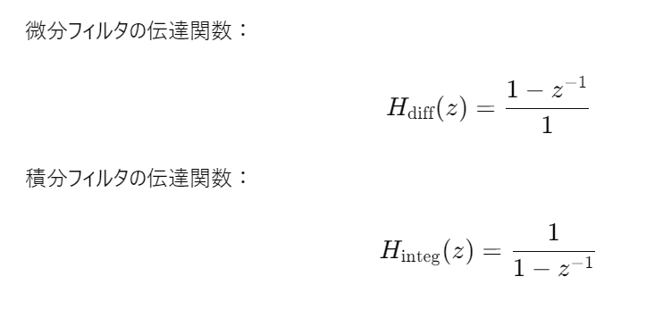
移動平均フィルタ
import numpy as np
import matplotlib.pyplot as plt

# 入力信号の関数
def input_signal(n):
    return 2 + 3 * (n - 1)

# 移動平均フィルタの伝達関数
def moving_average_filter(x, window_size):
    weights = np.ones(window_size) / window_size
    return np.convolve(x, weights, mode='valid')

# プロットするデータ点の数
num_points = 100

# 入力信号の作成
T_values = np.arange(1, num_points + 1)
a_values = np.array([input_signal(n) for n in T_values])

# 移動平均フィルタの適用
window_size = 5  # フィルタのウィンドウサイズ
filtered_values = moving_average_filter(a_values, window_size)

# プロット
plt.plot(T_values[:len(a_values)], a_values, label='Input Signal', linestyle='--')
plt.plot(T_values[:len(filtered_values)], filtered_values, label='Filtered Signal')
plt.xlabel('T')
plt.ylabel('Value')
plt.title('Input Signal vs Filtered Signal')
plt.legend()
plt.grid(True)
plt.show()
import numpy as np
import matplotlib.pyplot as plt
from scipy import signal
# サンプリング周波数
fs = 1000 # Hz
# デジタルフィルタの係数
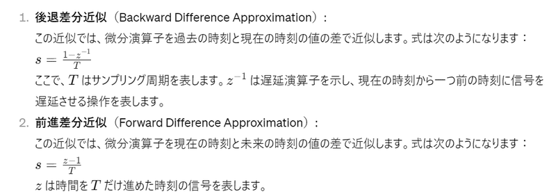
b_diff = [1, -1] # 微分フィルタの分子係数
a_diff = [1] # 微分フィルタの分母係数
b_integ = [1] # 積分フィルタの分子係数
a_integ = [1, -1] # 積分フィルタの分母係数
# 周波数応答の計算
freqs, response_diff = signal.freqz(b_diff, a_diff, fs=fs) # 微分フィルタの周波数応答
freqs, response_integ = signal.freqz(b_integ, a_integ, fs=fs) # 積分フィルタの周波数応答
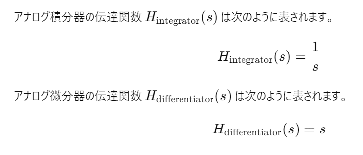
# アナログ積分器とアナログ微分器の周波数応答を定義
def analog_integrator(f):
return 1 / (2j * np.pi * f)
def analog_differentiator(f):
return 2j * np.pi * f
# 周波数範囲を設定
frequencies = np.logspace(0, 4, 1000)
# アナログフィルタの周波数応答を計算
integ_response = analog_integrator(frequencies)
diff_response = analog_differentiator(frequencies)
# プロット
plt.figure(figsize=(10, 12))
# 微分フィルタの周波数応答プロット
plt.subplot(3, 1, 1)
plt.plot(freqs, np.abs(response_diff), color='blue')
plt.title('デジタルフィルタの周波数応答 (微分フィルタ)')
plt.ylabel('ゲイン')
plt.xlabel('周波数 [Hz]')
plt.grid(True) # グリッドを表示
# 積分フィルタの周波数応答プロット
plt.subplot(3, 1, 2)
plt.plot(freqs, np.abs(response_integ), color='orange')
plt.ylabel('ゲイン')
plt.xlabel('周波数 [Hz]')
plt.grid(True) # グリッドを表示
# アナログ積分器とアナログ微分器の周波数応答プロット
plt.subplot(3, 1, 3)
plt.plot(frequencies, np.abs(integ_response), color='green')
plt.plot(frequencies, np.abs(diff_response), linestyle='--', color='red')
plt.xscale('log')
plt.yscale('log')
plt.title('アナログ積分器とアナログ微分器の周波数応答')
plt.xlabel('周波数 [Hz]')
plt.ylabel('ゲイン')
plt.grid(True)
plt.tight_layout()
plt.show()
RCL回路のPID制御 入力はのこぎり波
import numpy as np
import matplotlib.pyplot as plt
from scipy import signal

# 関数定義
def G(s, L, R, C):
    return (s*L + R + 1/(s*C))

def input_signal(t):
    return signal.sawtooth(2 * np.pi * 0.5 * t)

def input_signal_transform(s):
    return 1/s

def G_transform(s, L, R, C):
    return G(s, L, R, C)

def inverse_laplace_transform(s_domain, Y_s):
    return np.real(np.fft.ifft(Y_s))

def bode_plot(w, H):
    plt.figure()
    plt.subplot(2, 1, 1)
    plt.semilogx(w, 20 * np.log10(abs(H)))
    plt.title('Bode Plot')
    plt.ylabel('Magnitude (dB)')
    plt.subplot(2, 1, 2)
    plt.semilogx(w, np.angle(H) * 180 / np.pi)
    plt.xlabel('Frequency (rad/s)')
    plt.ylabel('Phase (degrees)')
    plt.show()

# パラメータ設定
L = 1.0
R = 1.0
C = 1.0

# 時間と周波数の設定
t = np.linspace(0, 10, num=1000)
s_domain = np.logspace(-1, 2, 1000)

# 入力信号と入力信号のラプラス変換のプロット
input_sig = input_signal(t)
input_sig_transform = input_signal_transform(s_domain)
plt.figure()
plt.subplot(2, 1, 1)
plt.plot(t, input_sig)
plt.title('Input Signal')
plt.xlabel('Time')
plt.ylabel('Amplitude')
plt.subplot(2, 1, 2)
plt.plot(s_domain, input_sig_transform)
plt.title('Transformed Input Signal')
plt.xlabel('Frequency (rad/s)')
plt.ylabel('Amplitude')
plt.show()

# G(s)とその変換のプロット
G_s = G_transform(s_domain, L, R, C)
plt.figure()
plt.subplot(2, 1, 1)
plt.plot(s_domain, np.abs(G_s))
plt.title('Magnitude of G(s)')
plt.xlabel('Frequency (rad/s)')
plt.ylabel('Magnitude')
plt.subplot(2, 1, 2)
plt.plot(s_domain, np.angle(G_s))
plt.title('Phase of G(s)')
plt.xlabel('Frequency (rad/s)')
plt.ylabel('Phase')
plt.show()

# G(s) * 入力(s)のプロット
output_s = G_s * input_sig_transform
plt.figure()
plt.subplot(2, 1, 1)
plt.plot(s_domain, np.abs(output_s))
plt.title('Magnitude of G(s) * Input(s)')
plt.xlabel('Frequency (rad/s)')
plt.ylabel('Magnitude')
plt.subplot(2, 1, 2)
plt.plot(s_domain, np.angle(output_s))
plt.title('Phase of G(s) * Input(s)')
plt.xlabel('Frequency (rad/s)')
plt.ylabel('Phase')
plt.show()

# 逆ラプラス変換と出力信号のプロット
output_time = inverse_laplace_transform(s_domain, output_s)
plt.figure()
plt.plot(t, output_time)
plt.title('Output Signal')
plt.xlabel('Time')
plt.ylabel('Amplitude')
plt.show()

# ボード線図のプロット
w, mag, phase = signal.bode((L, [R, 1/C]))
bode_plot(w, mag + phase * 1j)
チェビシェフフィルタとベッセルフィルタ
import numpy as np
import matplotlib.pyplot as plt
from scipy.signal import freqs, cheby1, bessel

# チェビシェフフィルタの設計
order = 5  # フィルタ次数
ripple = 1  # リプルの最大値 [dB]
cutoff_freq = 1000  # カットオフ周波数 [Hz]
nyquist_freq = 2 * cutoff_freq  # ナイキスト周波数

b, a = cheby1(order, ripple, cutoff_freq, 'low', analog=True)
w, h = freqs(b, a, worN=np.logspace(0, 5, 1000))

plt.figure()
plt.semilogx(w, 20 * np.log10(abs(h)))
plt.title('Chebyshev Filter Frequency Response')
plt.xlabel('Frequency [Hz]')
plt.ylabel('Gain [dB]')
plt.grid()

# ベッセルフィルタの設計
b_bessel, a_bessel = bessel(order, cutoff_freq, 'low', analog=True)
w_bessel, h_bessel = freqs(b_bessel, a_bessel, worN=np.logspace(0, 5, 1000))

plt.figure()
plt.semilogx(w_bessel, 20 * np.log10(abs(h_bessel)))
plt.title('Bessel Filter Frequency Response')
plt.xlabel('Frequency [Hz]')
plt.ylabel('Gain [dB]')
plt.grid()

plt.show()
FIRフィルター IIRフィルター
import numpy as np
import matplotlib.pyplot as plt
from scipy import signal

# 伝達関数の分子と分母の係数
numerator = [1, 2, 1]  # A + Bz^(-1) + Cz^(-2)
denominator = [1, 0.5, 0.3]  # 1 + Dz^(-1) + Ez^(-2)

# 角周波数の範囲を設定
w = np.logspace(-2, 1, 1000)  # 角周波数の範囲 (0.01から10まで)

# 周波数応答を計算
w, H = signal.freqz(numerator, denominator, worN=w)

# ゲイン特性と位相特性を計算
gain = np.abs(H)
phase = np.angle(H)

# ゲイン特性のプロット
plt.figure(figsize=(8, 6))
plt.subplot(2, 1, 1)
plt.plot(w, gain)
plt.xscale('log')
plt.title('Frequency Response')
plt.xlabel('Frequency [rad/s]')
plt.ylabel('Gain')

# 位相特性のプロット
plt.subplot(2, 1, 2)
plt.plot(w, phase)
plt.xscale('log')
plt.title('Phase Response')
plt.xlabel('Frequency [rad/s]')
plt.ylabel('Phase [radians]')

plt.tight_layout()
plt.show()
import numpy as np
import matplotlib.pyplot as plt

def moving_average_impulse_response(N):
    # 移動平均フィルタのインパルス応答 (係数は 1/N)
    h = np.ones(N) / N
    return h

def plot_frequency_response(h):
    # インパルス応答のフーリエ変換を計算
    H = np.fft.fft(h)

    # 周波数応答のプロット
    plt.figure(figsize=(8, 6))
    plt.plot(np.abs(H))
    plt.title('Frequency Response of Moving Average Filter')
    plt.xlabel('Frequency (Hz)')
    plt.ylabel('Magnitude')
    plt.grid(True)
    plt.show()

# ウィンドウサイズ N を指定
N = 16

# 移動平均フィルタのインパルス応答を取得
h = moving_average_impulse_response(N)

# 周波数特性をプロット
plot_frequency_response(h)
水と速度ポテンシャルA
import sympy as sp

# 変数の定義
x, y, z = sp.symbols('x y z')

# 速度ポテンシャル
A = x * y * z**2

# Aをx, y, zで偏微分
dA_dx = sp.diff(A, x)
dA_dy = sp.diff(A, y)
dA_dz = sp.diff(A, z)

# 水粒子速度
u = dA_dx
v = dA_dy
w = dA_dz

# 結果の表示
print("速度ポテンシャル A(x, y, z) =", A)
print("水粒子速度 u =", u)
print("水粒子速度 v =", v)
print("水粒子速度 w =", w)
import numpy as np
import matplotlib.pyplot as plt

def wave(amplitude, frequency, phase, time):
    return amplitude * np.sin(2 * np.pi * frequency * time + phase)

# パラメータ設定
duration = 2  # 秒
sampling_rate = 1000  # サンプリングレート
time = np.linspace(0, duration, int(duration * sampling_rate))

# 入力波形のパラメータ
input_amplitude = 1.0
input_frequency = 2.0
input_phase = 0

# 出力波形のパラメータ
output_amplitude = 0.5
output_frequency = 3.0
output_phase = np.pi / 2

# 入力波形と出力波形を生成
input_waveform = wave(input_amplitude, input_frequency, input_phase, time)
output_waveform = wave(output_amplitude, output_frequency, output_phase, time)

# グラフ表示
plt.figure(figsize=(10, 6))

# 入力波形をプロット
plt.plot(time, input_waveform, label='入力波形', color='blue')

# 出力波形をプロット
plt.plot(time, output_waveform, label='出力波形', color='red')

plt.title('入力波形と出力波形')
plt.xlabel('時間 (秒)')
plt.ylabel('振幅')
plt.legend()
plt.grid(True)
plt.show()
import math

def venturi_meter(area1, area2, velocity1):
    """
    ベンチュリメーターを使って流体の速度と圧力差を計算する関数

    Parameters:
        area1 (float): 収縮部前の管の断面積 (m^2)
        area2 (float): 収縮部の管の断面積 (m^2)
        velocity1 (float): 収縮部前の流体の速度 (m/s)

    Returns:
        velocity2 (float): 収縮部での流体の速度 (m/s)
        pressure_difference (float): 収縮部を通る際の圧力差 (Pa)
    """
    velocity2 = (area1 / area2) * velocity1
    pressure_difference = 0.5 * (velocity2**2 - velocity1**2)
    return velocity2, pressure_difference

def bernoulli_theorem(density, velocity1, pressure1, height1, height2):
    """
    ベルヌーイの定理を適用して点2の圧力を計算する関数

    Parameters:
        density (float): 流体の密度 (kg/m^3)
        velocity1 (float): 点1での流体の速度 (m/s)
        pressure1 (float): 点1での流体の圧力 (Pa)
        height1 (float): 点1の高さ (m)
        height2 (float): 点2の高さ (m)

    Returns:
        pressure2 (float): 点2での流体の圧力 (Pa)
    """
    pressure2 = pressure1 + 0.5 * density * (velocity1**2) + density * 9.81 * (height1 - height2)
    return pressure2

# 例としての値
area1 = 0.01  # m^2
area2 = 0.005  # m^2
velocity1 = 10  # m/s
density = 1000  # kg/m^3(水の場合)
pressure1 = 100000  # Pa(1気圧)
height1 = 10  # m
height2 = 5  # m

# ベンチュリメーターを使って速度と圧力差を計算
velocity2, pressure_difference = venturi_meter(area1, area2, velocity1)

print("収縮部での速度(m/s):", velocity2)
print("収縮部を通る際の圧力差(Pa):", pressure_difference)

# ベルヌーイの定理を使って点2での圧力を計算
pressure2 = bernoulli_theorem(density, velocity1, pressure1, height1, height2)
print("点2での圧力(Pa):", pressure2)
スミスチャート
http://udonyanocurry.seesaa.net/article/464049976.htm
この記事が気に入ったらサポートをしてみませんか?