電気電子回路

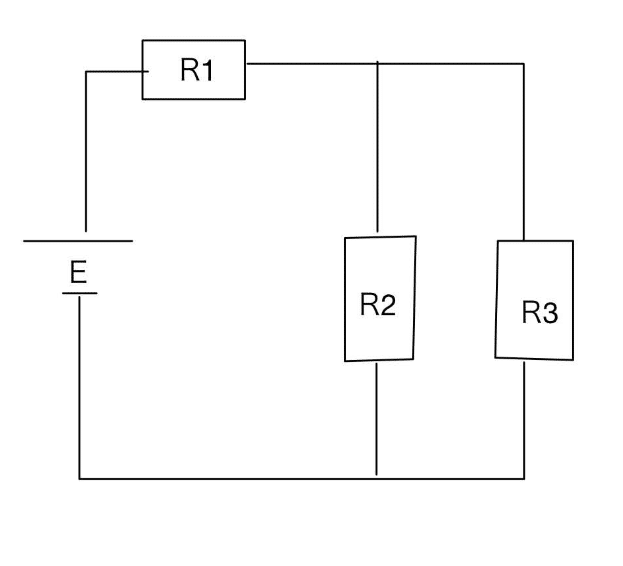
# 定数の設定
R1 = 5  # 抵抗値1 (オーム)
R2 = 10 # 抵抗値2 (オーム)
R3 = 15 # 抵抗値3 (オーム)
E = 20  # 電圧値 (ボルト)

# 分母の計算
denominator = R1 * R2 + R1 * R3 + R2 * R3

# I2およびI3の計算
I2 = (R3 * E) / denominator
I3 = (R2 * E) / denominator

# 結果の表示
print("I2 =", I2, "A")
print("I3 =", I3, "A")
import numpy as np
import matplotlib.pyplot as plt

# 与えられた値
R1 = 1
R2 = 2
R3 = 3
R4 = 4
R5 = 5
E = 5

# 係数行列の作成
A = np.array([[R1+R3+R5, -R5, -R3],
              [-R5, R2+R4+R5, -R4],
              [-R3, -R4, R3+R4]])

# 定数項の作成
B = np.array([E, 0, 0])

# 方程式を解く
I = np.linalg.solve(A, B)

# 結果の表示
print("I1 =", I[0])
print("I2 =", I[1])
print("I3 =", I[2])

# グラフのプロット
labels = ['I1', 'I2', 'I3']
plt.bar(labels, I)
plt.ylabel('Current (A)')
plt.title('Current Flow')
plt.show()
import numpy as np
import matplotlib.pyplot as plt

# 定数定義
A = 10000
beta = 0.5  # 任意の値を設定

# v(t) = sin(omega * t) を定義
def v(t, omega):
    return np.sin(omega * t)

# (A/(1+A*beta)) を計算する関数
def calculate_A_over_1_plus_A_beta(A, beta):
    return A / (1 + A * beta)

# v(t) * (A/(1+A*beta)) を計算する関数
def calculate_v_times_A_over_1_plus_A_beta(t, omega, A, beta):
    return v(t, omega) * calculate_A_over_1_plus_A_beta(A, beta)

# 1/ beta を計算する関数
def calculate_inverse_beta(beta):
    return 1 / beta

# 時間配列の作成
t = np.linspace(0, 2*np.pi, 1000)  # 0から2πまでの1000点

# omega の選択(任意)
omega = 1

# v(t) と (A/(1+A*beta))×v(t) の計算
v_t = v(t, omega)
v_times_A_over_1_plus_A_beta = calculate_v_times_A_over_1_plus_A_beta(t, omega, A, beta)

# プロット
plt.figure(figsize=(10, 5))

# v(t) のプロット
plt.subplot(2, 1, 1)
plt.plot(t, v_t, label='v(t)')
plt.title('v(t)')
plt.xlabel('Time')
plt.ylabel('Amplitude')
plt.legend()

# (A/(1+A*beta))×v(t) のプロット
plt.subplot(2, 1, 2)
plt.plot(t, v_times_A_over_1_plus_A_beta, label='(A/(1+A*beta))×v(t)')
plt.title('(A/(1+A*beta))×v(t)')
plt.xlabel('Time')
plt.ylabel('Amplitude')
plt.legend()

plt.tight_layout()
plt.show()

# 1/beta の計算と表示
inverse_beta = calculate_inverse_beta(beta)
print("1/beta =", inverse_beta)
A = 10000
R1 = 5
R2 = 10

# 非反転オープンループゲインの計算
non_inverting_gain = A / (1 + R2 * A / (R1 + R2))
print("非反転オープンループゲイン:", non_inverting_gain)

# 反転オープンループゲインの計算
inverting_gain = -R1 / (((R1 + R2) / A) + R2)
print("反転オープンループゲイン:", inverting_gain)
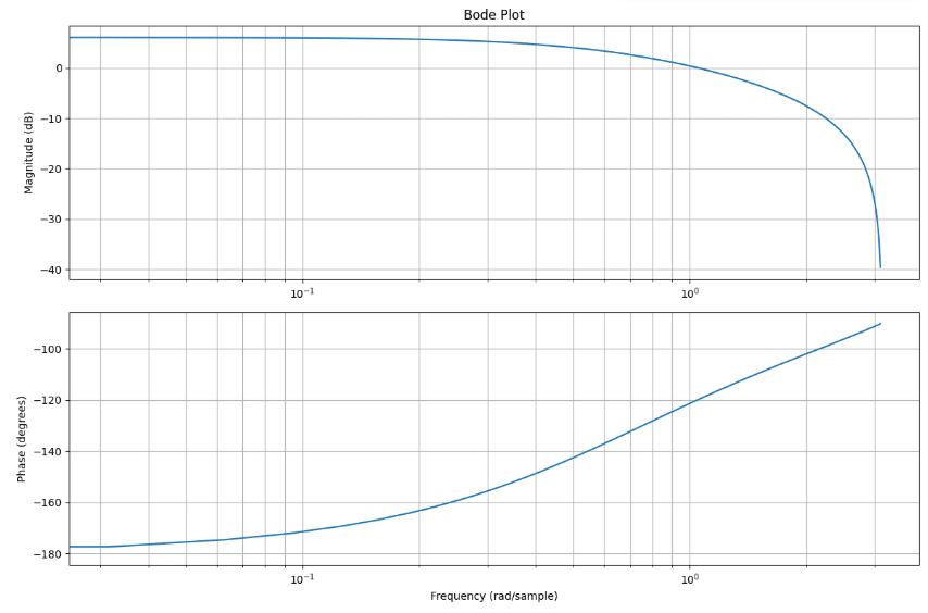
import numpy as np
import matplotlib.pyplot as plt
from scipy import signal

# 定数を設定 (例: T1=1, T2=2)
T1 = 1
T2 = 2

# 伝達関数を定義
numerator = [T2, 0]    # 分子の係数 (T2s)
denominator = [T1, 1]  # 分母の係数 (T1s + 1)

system = signal.TransferFunction(numerator, denominator)

# 周波数範囲を指定
frequencies = np.logspace(-2, 2, 500)  # 0.01から100までの対数スケールの周波数範囲

# Bodeプロットを計算
w, mag, phase = signal.bode(system, frequencies)

# ボード線図をプロット
plt.figure()

# 振幅特性をプロット
plt.subplot(2, 1, 1)
plt.semilogx(w, mag)    # 周波数軸を対数スケールでプロット
plt.title('Bode Plot')
plt.ylabel('Magnitude (dB)')
plt.grid(which='both', linestyle='--', linewidth=0.5)

# 位相特性をプロット
plt.subplot(2, 1, 2)
plt.semilogx(w, phase)  # 周波数軸を対数スケールでプロット
plt.ylabel('Phase (degrees)')
plt.xlabel('Frequency (rad/s)')
plt.grid(which='both', linestyle='--', linewidth=0.5)

plt.tight_layout()
plt.show()
1次進み遅れ系×1次遅れ系伝達関数
A(1+s/c)/((1+s/a)(1+s/b))
import numpy as np
import matplotlib.pyplot as plt
from scipy.signal import TransferFunction, bode

# パラメータの設定
a = 10.0
b = 100000.0
c = 100000000000.0

# 伝達関数の係数
num = [1, c]  # 分子 (1 + s/c)
den = [1, a+b, a*b]  # 分母 ((1 + s/a)(1 + s/b))

# 伝達関数オブジェクトの作成
system = TransferFunction(num, den)

# 周波数応答の計算
w, mag, phase = bode(system)

# ボード線図のプロット
plt.figure()

# 振幅応答
plt.subplot(2, 1, 1)
plt.semilogx(w, mag)  # 振幅をdBでプロット
plt.title('Bode Plot')
plt.xlabel('Frequency [rad/s]')
plt.ylabel('Magnitude [dB]')
plt.grid(which='both', linestyle='--', linewidth=0.5)

# 位相応答
plt.subplot(2, 1, 2)
plt.semilogx(w, phase)  # 位相を度でプロット
plt.xlabel('Frequency [rad/s]')
plt.ylabel('Phase [degrees]')
plt.grid(which='both', linestyle='--', linewidth=0.5)

plt.tight_layout()
plt.show()
import numpy as np
import matplotlib.pyplot as plt

# 定数の設定
mu = 100e-6  # 運動度 (cm^2/Vs)
Cox = 1e-8   # 酸化物容量 (F/cm^2)
W = 1e-4     # チャネル幅 (cm)
L = 1e-4     # チャネル長 (cm)
Vth = 1.0    # 閾値電圧 (V)
lambda_ = 0.1  # チャネル長変調係数
VDS = 5.0    # ドレイン-ソース間電圧 (V)

# ID1のプロット (VGS vs ID1)
VGS = np.linspace(0, 5, 100)  # VGSの範囲
ID1 = 0.5 * mu * Cox * (W/L) * ((VGS - Vth) ** 2) * (1 + lambda_ * VDS)
ID1[VGS < Vth] = 0  # VGSがVthより小さい場合はID1が0になる

plt.figure()
plt.plot(VGS, ID1)
plt.title('VGS vs ID1')
plt.xlabel('VGS (V)')
plt.ylabel('ID1 (A)')
plt.grid(True)
plt.show()

# ID2のプロット (VDS vs ID2)
VDS = np.linspace(0, 5, 100)  # VDSの範囲
VGS = 3.0  # 固定VGS (V)
ID2 = 0.5 * mu * Cox * (W/L) * ((VGS - Vth) ** 2) * (1 + lambda_ * VDS)
ID2[VGS < Vth] = 0  # VGSがVthより小さい場合はID2が0になる

plt.figure()
plt.plot(VDS, ID2)
plt.title('VDS vs ID2')
plt.xlabel('VDS (V)')
plt.ylabel('ID2 (A)')
plt.grid(True)
plt.show()
https://www.ritsumei.ac.jp/se/re/fujinolab/FujinolabHP_old/semicon/semicon12.pdf
import math

def 有効ゲート電圧(ID, W, L, μ, Cox):
    V_eff = math.sqrt((2 * ID) / (μ * Cox * (W / L)))
    return V_eff

def 相互コンダクタンス(ID, W, L, μ, Cox):
    V_eff = 有効ゲート電圧(ID, W, L, μ, Cox)
    gm = 2 * ID / V_eff
    return gm

# 例としての使用
ID = 1e-3  # ドレイン電流(アンペア)
W = 10e-6  # チャネル幅(メートル)
L = 1e-6   # チャネル長さ(メートル)
μ = 600e-4 # チャネル移動度(m^2/V*s)
Cox = 3.45e-6 # 単位面積当たりの容量(F/m^2)

V_eff = 有効ゲート電圧(ID, W, L, μ, Cox)
gm = 相互コンダクタンス(ID, W, L, μ, Cox)

print("有効ゲート電圧:", V_eff, "ボルト")
print("相互コンダクタンス:", gm, "ジーメンス")
https://akizukidenshi.com/goodsaffix/NJM4250_j.
https://akizukidenshi.com/goodsaffix/NJM4250_j.
https://www.ti.com/jp/lit/ds/symlink/tlv9064-q1.pdf
import numpy as np
import matplotlib.pyplot as plt

# Given constants
mu = 200e-4   # Mobility (m^2/V·s)
Cox = 10e-9   # Oxide capacitance (F/m^2)
W = 10e-6     # Width of the MOSFET (m)
L = 1e-6      # Length of the MOSFET (m)
Vth = 1       # Threshold voltage (V)
VA = 100      # Early voltage (V)
VDS = 5       # Drain-source voltage (V)

# Generate VG values
VG = np.linspace(0, 5, 500)

# Calculate gm
def calculate_gm(VG, mu, Cox, W, L, Vth, VDS, VA):
    gm = np.zeros_like(VG)
    for i, VGS in enumerate(VG):
        if VGS > Vth:
            gm[i] = mu * Cox * (W / L) * (VGS - Vth) * (1 + VDS / VA)
    return gm

gm = calculate_gm(VG, mu, Cox, W, L, Vth, VDS, VA)

# Plot gm vs VG
plt.figure(figsize=(10, 6))
plt.plot(VG, gm, label='$g_m$ vs $V_G$', color='b')
plt.xlabel('$V_G$ (V)')
plt.ylabel('$g_m$ (S)')
plt.title('Transconductance $g_m$ vs Gate Voltage $V_G$')
plt.grid(True)
plt.legend()
plt.show()
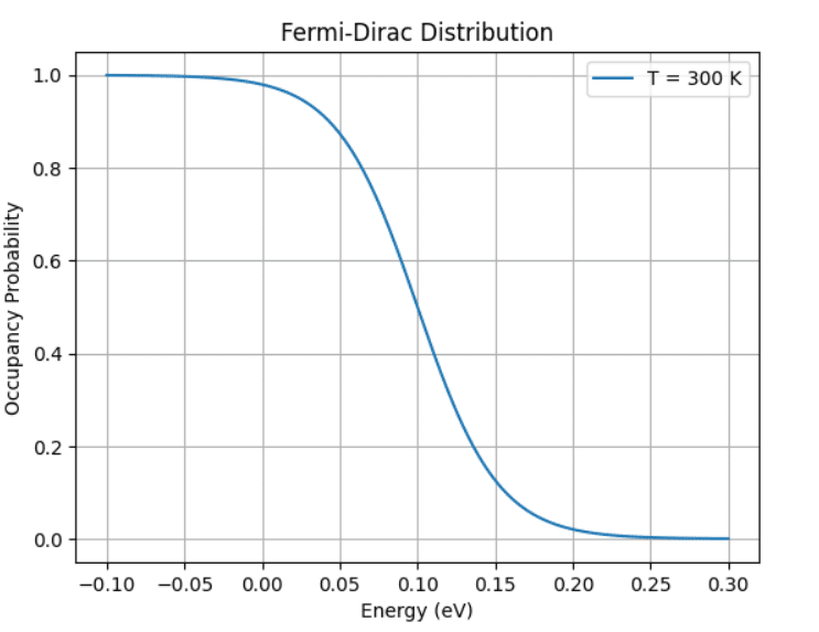
import numpy as np
import matplotlib.pyplot as plt

# 定数の定義
k_B = 8.617333262145e-5  # eV/K (ボルツマン定数)

def fermi_dirac(E, E_F, T):
    """
    フェルミディラック分布関数を計算する関数

    Parameters:
    E : float or ndarray
        エネルギー (eV)
    E_F : float
        フェルミエネルギー (eV)
    T : float
        絶対温度 (K)

    Returns:
    f(E) : float or ndarray
        エネルギー E における占有確率
    """
    return 1 / (np.exp((E - E_F) / (k_B * T)) + 1)

# パラメータの設定
E_F = 0.1  # フェルミエネルギー (eV)
T = 300  # 絶対温度 (K)

# エネルギー範囲の設定
E = np.linspace(-0.1, 0.3, 500)  # エネルギー (eV)

# フェルミディラック分布関数の計算
f_E = fermi_dirac(E, E_F, T)

# グラフのプロット
plt.plot(E, f_E, label=f'T = {T} K')
plt.xlabel('Energy (eV)')
plt.ylabel('Occupancy Probability')
plt.title('Fermi-Dirac Distribution')
plt.legend()
plt.grid(True)
plt.show()
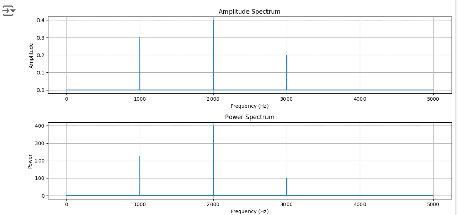
import numpy as np
import matplotlib.pyplot as plt

# サンプリング周波数と時間ベクトルの設定
fs = 10000  # サンプリング周波数(Hz)
t = np.arange(0, 1, 1/fs)  # 時間ベクトル(1秒分のデータ)

# 与えられた信号の生成
f_t = 0.3 * np.sin(2 * np.pi * 1000 * t) + 0.4 * np.sin(2 * np.pi * 2000 * t) + 0.2 * np.sin(2 * np.pi * 3000 * t)

# FFTの計算
f_fft = np.fft.fft(f_t)
N = len(f_t)
f_fft = f_fft[:N//2]  # FFTの前半分だけを使用(対称性を利用)
freq = np.fft.fftfreq(N, 1/fs)[:N//2]  # 周波数ベクトル

# 振幅スペクトルの計算
amplitude_spectrum = np.abs(f_fft) / N * 2  # 振幅スペクトル

# パワースペクトルの計算
power_spectrum = np.abs(f_fft) ** 2 / N  # パワースペクトル

# 結果のプロット
plt.figure(figsize=(12, 6))

# 振幅スペクトルのプロット
plt.subplot(2, 1, 1)
plt.plot(freq, amplitude_spectrum)
plt.title('Amplitude Spectrum')
plt.xlabel('Frequency (Hz)')
plt.ylabel('Amplitude')
plt.grid()

# パワースペクトルのプロット
plt.subplot(2, 1, 2)
plt.plot(freq, power_spectrum)
plt.title('Power Spectrum')
plt.xlabel('Frequency (Hz)')
plt.ylabel('Power')
plt.grid()

plt.tight_layout()
plt.show()
import numpy as np
import matplotlib.pyplot as plt
from scipy.fft import fft

# Parameters
Ts = 5  # 5 seconds
Fs = 8192  # Sampling frequency 8192 Hz

# Time vector for sampling
t = np.linspace(0, Ts, Ts * Fs, endpoint=False)

# Frequencies
hz1 = 1000
hz2 = 2000
hz3 = 3000

# Signals
y1 = 0.3 * np.sin(2 * np.pi * hz1 * t)  # 1 kHz
y2 = 0.4 * np.sin(2 * np.pi * hz2 * t)  # 2 kHz
y3 = 0.2 * np.sin(2 * np.pi * hz3 * t)  # 3 kHz

# Combined signal
all_signal = y1 + y2 + y3

# Play sound (optional, requires sounddevice library)
# import sounddevice as sd
# sd.play(all_signal, Fs)
# sd.wait()

# FFT
f = np.linspace(0, Fs, 8192, endpoint=False)
fft_y = fft(all_signal[:8192])

# Plot
plt.plot(f, np.abs(fft_y) / 4096, linewidth=2.0)
plt.axis([0, 4096, 0, 1.0])
plt.show()

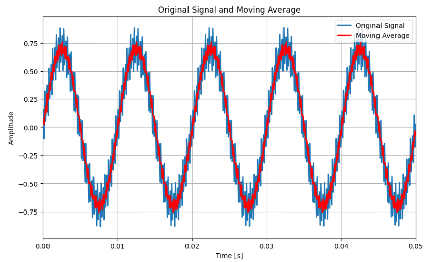
import numpy as np
import matplotlib.pyplot as plt

# Sampling frequency
Fs = 10000

# Time vector
t = np.linspace(0, 1, Fs)

# Signals
y1 = 0.7 * np.sin(2 * np.pi * 100 * t)
y2 = 0.2 * np.sin(2 * np.pi * 4000 * t)

# Combined signal
y = y1 + y2

# Initialize moving average array
y_mave = np.zeros(Fs)
y_mave[0] = 0

# Compute moving average
for n in range(1, Fs):
    y_mave[n] = (y[n] + y[n-1]) / 2

# Plotting the signals
plt.figure(figsize=(10, 6))
plt.plot(t, y, label='Original Signal', linewidth=2.0)
plt.plot(t, y_mave, 'r', label='Moving Average', linewidth=2.0)
plt.xlim(0, 0.05)
plt.xlabel('Time [s]')
plt.ylabel('Amplitude')
plt.legend()
plt.grid(True)
plt.title('Original Signal and Moving Average')
plt.show()
import numpy as np
import matplotlib.pyplot as plt

def compute_lsb(FS, N):
    """
    Compute the Least Significant Bit (LSB).

    Parameters:
    FS (float): Full Scale range
    N (int): Number of bits

    Returns:
    float: The value of the Least Significant Bit (LSB)
    """
    return FS / (2**N - 1)

def generate_signal(A, T, theta, num_points):
    """
    Generate a sinusoidal signal y(t, θ) = A * sin(2πt/T + θ).

    Parameters:
    A (float): Amplitude of the signal
    T (float): Period of the signal
    theta (float): Phase of the signal in radians
    num_points (int): Number of points in the signal

    Returns:
    np.ndarray: Array containing the signal values
    np.ndarray: Array containing the time values
    """
    t = np.linspace(0, T, num_points)
    y = A * np.sin(2 * np.pi * t / T + theta)
    return t, y

# Example usage:
if __name__ == "__main__":
    # Parameters for LSB computation
    FS = 10.0  # Full Scale range
    N = 8      # Number of bits
    lsb = compute_lsb(FS, N)
    print(f"Least Significant Bit (LSB): {lsb}")

    # Parameters for signal generation
    A = 1.0            # Amplitude
    T = 1.0            # Period
    theta = np.pi / 4  # Phase in radians
    num_points = 1000  # Number of points

    t, y = generate_signal(A, T, theta, num_points)

    # Plot the signal
    plt.figure(figsize=(10, 6))
    plt.plot(t, y)
    plt.title("Sinusoidal Signal")
    plt.xlabel("Time (t)")
    plt.ylabel("Amplitude (y)")
    plt.grid(True)
    plt.show()
import numpy as np
import matplotlib.pyplot as plt

# パラメータ設定
fc = 100
Fs = 400
wc = 2 * np.pi * (fc / Fs)

# インパルス応答を計算する関数
def h(k):
    if k == 0:
        return wc / np.pi
    else:
        return np.sin(wc * k) / (np.pi * k)

# kの範囲を設定
k_values = np.arange(-20, 21)

# インパルス応答を計算
h_values = np.array([h(k) for k in k_values])

# 結果をプロット
plt.stem(k_values, h_values, use_line_collection=True)
plt.xlabel('k')
plt.ylabel('h(k)')
plt.title('Impulse Response of Low-Pass Filter')
plt.grid(True)
plt.show()

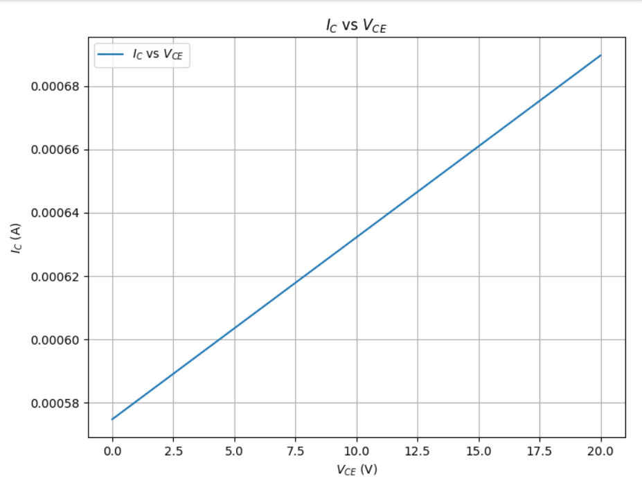
import numpy as np
import matplotlib.pyplot as plt

# 定数の定義
q = 1.60219e-19  # 電気素量 (C)
k = 1.38066e-23  # ボルツマン定数 (J/K)
T = 300          # 絶対温度 (K)

# パラメータの定義
I_S = 1e-15      # 飽和電流 (A)
V_A = 100        # アーリー電圧 (V)
V_BE = 0.7       # ベース-エミッタ電圧 (V)

# VCEの範囲を設定
VCE = np.linspace(0, 20, 400)

# ICを計算する
IC = I_S * np.exp(q * V_BE / (k * T)) * (1 + VCE / V_A)

# グラフの描画
plt.figure(figsize=(8, 6))
plt.plot(VCE, IC, label='$I_C$ vs $V_{CE}$')
plt.xlabel('$V_{CE}$ (V)')
plt.ylabel('$I_C$ (A)')
plt.title('$I_C$ vs $V_{CE}$')
plt.legend()
plt.grid(True)
plt.show()
import numpy as np
import matplotlib.pyplot as plt
from scipy import signal

# パラメータの設定
R = 0.5  # 例として設定、適宜変更
theta = np.pi / 4  # 例として設定、適宜変更

# 伝達関数の係数の計算
b = [1]
a = [1, -2 * R * np.cos(theta), R**2]

# 周波数応答の計算
w, h = signal.freqz(b, a, worN=8000)

# 振幅と位相の計算
amplitude = 20 * np.log10(abs(h))
phase = np.angle(h, deg=True)

# ボード線図のプロット
fig, (ax1, ax2) = plt.subplots(2, 1, figsize=(10, 7))

# 振幅特性のプロット
ax1.plot(w / np.pi, amplitude)
ax1.set_title('Bode Plot')
ax1.set_ylabel('Magnitude (dB)')
ax1.grid()

# 位相特性のプロット
ax2.plot(w / np.pi, phase)
ax2.set_ylabel('Phase (degrees)')
ax2.set_xlabel('Normalized Frequency (×π rad/sample)')
ax2.grid()

plt.show()


FIR
import numpy as np
import matplotlib.pyplot as plt
from scipy import signal

# 伝達関数のパラメータを設定
a = 1.0  # ここで a の値を設定します
b = 1.0  # ここで b の値を設定します

# 伝達関数の係数を設定
numerator_coeffs = [a, 1]       # 分子の係数
denominator_coeffs = [1, -a*b - b] # 分母の係数

# 伝達関数を作成
system = signal.dlti(numerator_coeffs, denominator_coeffs)

# 周波数応答を計算
w, mag, phase = signal.dbode(system)

# ボード線図をプロット
plt.figure(figsize=(12, 8))

# 利得プロット
plt.subplot(2, 1, 1)
plt.semilogx(w, mag)    # 周波数を対数スケールでプロット
plt.title('Bode Plot')
plt.ylabel('Magnitude (dB)')
plt.grid(which='both', axis='both')

# 位相プロット
plt.subplot(2, 1, 2)
plt.semilogx(w, phase)  # 周波数を対数スケールでプロット
plt.xlabel('Frequency (rad/sample)')
plt.ylabel('Phase (degrees)')
plt.grid(which='both', axis='both')

plt.tight_layout()
plt.show()
import numpy as np
import matplotlib.pyplot as plt

# サンプルレートとサンプル数
Fs = 1000  # サンプリング周波数 (Hz)
T = 1.0 / Fs  # サンプリング間隔
N = 1000  # サンプル数
t = np.linspace(0.0, N*T, N)  # 時間軸

# 波形の周波数
f = 5  # 波形の周波数 (Hz)

# 正弦波
sin_wave = np.sin(2.0 * np.pi * f * t)

# 三角波
triangle_wave = 2 * np.abs(2 * (t*f - np.floor(t*f + 0.5))) - 1

# 短形波 (矩形波)
square_wave = np.sign(np.sin(2.0 * np.pi * f * t))

# のこぎり波
sawtooth_wave = 2 * (t*f - np.floor(t*f + 0.5))

# FFT の計算
def compute_fft(wave):
    fft_values = np.fft.fft(wave)
    fft_freqs = np.fft.fftfreq(N, T)
    return fft_freqs, np.abs(fft_values)

# 波形のリスト
waves = [sin_wave, triangle_wave, square_wave, sawtooth_wave]
wave_names = ['Sine Wave', 'Triangle Wave', 'Square Wave', 'Sawtooth Wave']

# プロット
fig, axes = plt.subplots(4, 2, figsize=(14, 12))

for i, wave in enumerate(waves):
    fft_freqs, fft_values = compute_fft(wave)

    # 波形のプロット
    axes[i, 0].plot(t, wave)
    axes[i, 0].set_title(wave_names[i])
    axes[i, 0].set_xlabel('Time (s)')
    axes[i, 0].set_ylabel('Amplitude')

    # FFTのプロット
    axes[i, 1].stem(fft_freqs[:N // 2], fft_values[:N // 2], basefmt=" ")
    axes[i, 1].set_title(f'{wave_names[i]} FFT')
    axes[i, 1].set_xlabel('Frequency (Hz)')
    axes[i, 1].set_ylabel('Magnitude')

plt.tight_layout()
plt.show()
import numpy as np
import matplotlib.pyplot as plt

# サンプルレートとサンプル数
Fs = 1000  # サンプリング周波数 (Hz)
T = 1.0 / Fs  # サンプリング間隔
N = 1000  # サンプル数
t = np.linspace(0.0, N*T, N)  # 時間軸

# 波形の周波数
f = 5  # 波形の周波数 (Hz)

# 方形パルス列
pulse_train = np.sign(np.sin(2.0 * np.pi * f * t))

# 単一の方形パルス
single_pulse = np.zeros_like(t)
pulse_duration = int(0.1 * N)  # 10%の期間だけ1
single_pulse[N//2 - pulse_duration//2 : N//2 + pulse_duration//2] = 1

# 2乗余弦パルス
cosine_squared_pulse = np.cos(np.pi * (t - 0.5)**2 * Fs / N)**2

# 白色雑音
white_noise = np.random.normal(0, 1, N)

# FFT の計算
def compute_fft(wave):
    fft_values = np.fft.fft(wave)
    fft_freqs = np.fft.fftfreq(N, T)
    return fft_freqs, np.abs(fft_values)

# 波形のリスト
waves = [pulse_train, single_pulse, cosine_squared_pulse, white_noise]
wave_names = ['Pulse Train', 'Single Pulse', 'Cosine Squared Pulse', 'White Noise']

# プロット
fig, axes = plt.subplots(4, 2, figsize=(14, 12))

for i, wave in enumerate(waves):
    fft_freqs, fft_values = compute_fft(wave)

    # 波形のプロット
    axes[i, 0].plot(t, wave)
    axes[i, 0].set_title(wave_names[i])
    axes[i, 0].set_xlabel('Time (s)')
    axes[i, 0].set_ylabel('Amplitude')

    # FFTのプロット
    axes[i, 1].stem(fft_freqs[:N // 2], fft_values[:N // 2], basefmt=" ", use_line_collection=True)
    axes[i, 1].set_title(f'{wave_names[i]} FFT')
    axes[i, 1].set_xlabel('Frequency (Hz)')
    axes[i, 1].set_ylabel('Magnitude')

plt.tight_layout()
plt.show()
import numpy as np
import matplotlib.pyplot as plt
from scipy import signal

# システムのパラメータ
R1 = 1
R2 = 2
C = 0.1

# 伝達関数の分子と分母
numerator = [R2]
denominator = [R1 * C, 1, R1 + R2, 1/R2]

# 伝達関数を作成
sys = signal.TransferFunction(numerator, denominator)

# ボード線図を計算
w, mag, phase = signal.bode(sys)

# ボード線図をプロット
plt.figure()
plt.subplot(2, 1, 1)
plt.semilogx(w, mag)
plt.title('Bode Plot - Magnitude')
plt.ylabel('Magnitude (dB)')
plt.grid()

plt.subplot(2, 1, 2)
plt.semilogx(w, phase)
plt.title('Bode Plot - Phase')
plt.xlabel('Frequency (rad/s)')
plt.ylabel('Phase (degrees)')
plt.grid()

plt.show()
import numpy as np
import matplotlib.pyplot as plt
from mpl_toolkits.mplot3d import Axes3D
# Constants
k = 1.38e-23 # Boltzmann constant (J/K)
T = 300 # Absolute temperature (K)
q = 1.6e-19 # Electron charge (C)
V_T = k * T / q # Thermal voltage (V)
# Device parameters
V_th = 0.7 # Threshold voltage (V)
n = 1.5 # Subthreshold slope factor
I_D0 = 1e-12 # Reference current (A)
# Setting the range for VGS and VDS
VGS = np.linspace(0, 1, 100) # Range from 0V to 1V
VDS = np.linspace(0, 1, 100) # Range from 0V to 1V
# Creating a mesh grid
VGS, VDS = np.meshgrid(VGS, VDS)
# Calculating the drain current in the weak inversion region
I_D = I_D0 * np.exp((VGS - V_th) / (n * V_T)) * (1 - np.exp(-VDS / V_T))
# Creating the 3D plot
fig = plt.figure()
ax = fig.add_subplot(111, projection='3d')
ax.plot_surface(VGS, VDS, I_D, cmap='viridis')
# Setting labels
ax.set_xlabel('VGS (V)')
ax.set_ylabel('VDS (V)')
ax.set_zlabel('ID (A)')
ax.set_title('MOSFET Weak Inversion Region Current')
# Displaying the plot
plt.show()
import numpy as np
import matplotlib.pyplot as plt

# パラメータ設定
IREF = 1  # リファレンス電流 (任意の値に設定できます)
beta_values = np.linspace(10, 1000, 100)  # βの範囲

# ICBを計算
ICB_values = IREF / (1 + 3 / beta_values)

# プロット
plt.figure(figsize=(10, 6))
plt.plot(beta_values, ICB_values, label='ICB vs β')
plt.xlabel('β')
plt.ylabel('ICB (IREF/(1+3/β))')
plt.title('ICB vs β')
plt.grid(True)
plt.legend()
plt.show()
import numpy as np
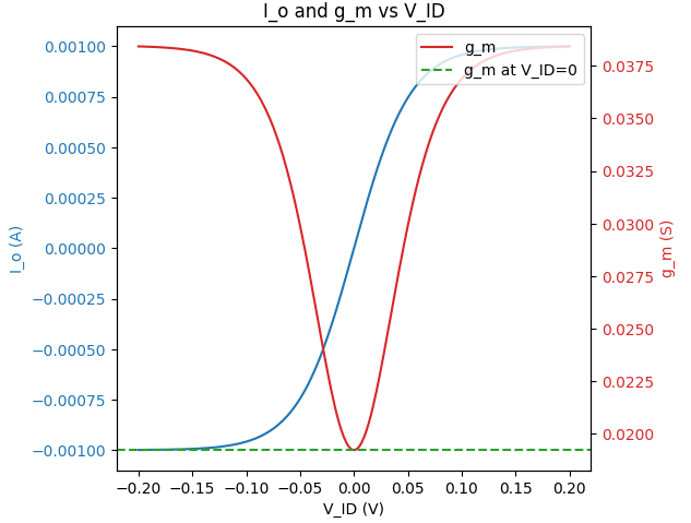
import matplotlib.pyplot as plt
# Define functions
def I_o(I_TAIL, V_ID, V_T):
term1 = I_TAIL / (1 + np.exp(-V_ID / V_T))
term2 = I_TAIL / (1 + np.exp(V_ID / V_T))
return term1 - term2
def g_m(I_TAIL, V_ID, V_T):
term1 = I_TAIL / (V_T * (1 + np.exp(-V_ID / V_T))**2)
term2 = I_TAIL / (V_T * (1 + np.exp(V_ID / V_T))**2)
return term1 + term2
# For V_ID = 0
def g_m_at_VID_zero(I_C, V_T):
return I_C / V_T
# Parameters
I_TAIL = 1e-3 # Example current in Amperes
V_T = 26e-3 # Thermal voltage at room temperature (approx 26mV)
V_ID_range = np.linspace(-0.2, 0.2, 400) # V_ID values from -0.2V to 0.2V
# Calculate I_o and g_m for the range of V_ID
I_o_values = I_o(I_TAIL, V_ID_range, V_T)
g_m_values = g_m(I_TAIL, V_ID_range, V_T)
# Calculate g_m at V_ID = 0
I_C = I_TAIL / 2
g_m_zero = g_m_at_VID_zero(I_C, V_T)
# Plotting
fig, ax1 = plt.subplots()
# Plot I_o
ax1.set_xlabel('V_ID (V)')
ax1.set_ylabel('I_o (A)', color='tab:blue')
ax1.plot(V_ID_range, I_o_values, label='I_o', color='tab:blue')
ax1.tick_params(axis='y', labelcolor='tab:blue')
# Create a twin Axes sharing the x-axis
ax2 = ax1.twinx()
# Plot g_m
ax2.set_ylabel('g_m (S)', color='tab:red')
ax2.plot(V_ID_range, g_m_values, label='g_m', color='tab:red')
ax2.tick_params(axis='y', labelcolor='tab:red')
# Highlight g_m at V_ID = 0
ax2.axhline(y=g_m_zero, color='tab:green', linestyle='--', label='g_m at V_ID=0')
ax2.legend(loc='upper right')
# Show plot
fig.tight_layout()
plt.title('I_o and g_m vs V_ID')
plt.show()
import numpy as np
import matplotlib.pyplot as plt

# 定数の定義
Im = 1  # 最大電流
R = 1   # 抵抗
C = 1   # コンデンサのキャパシタンス
ω = 1   # 角周波数
CR = C * R

# 時間の範囲を設定
t = np.linspace(0, 10, 1000)

# 入力電流の計算
I = Im * np.sin(ω * t)

# 出力電圧の計算
V = (R / np.sqrt(1 + (ω * CR)**2)) * Im * np.sin(ω * t - np.arctan(ω * CR))

# プロット
plt.plot(t, I, label='Input Current (I(t))')
plt.plot(t, V, label='Output Voltage (V(t))')
plt.xlabel('Time')
plt.ylabel('Amplitude')
plt.title('Input Current and Output Voltage')
plt.legend()
plt.grid(True)
plt.show()
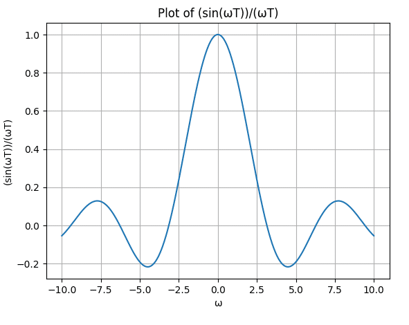
import numpy as np
import matplotlib.pyplot as plt

# ωの値の範囲を設定
omega_values = np.linspace(-10, 10, 10000)  # 0から10の範囲で1000点を生成

# 式の計算
function_values = np.sin(omega_values * 1) / (omega_values * 1)  # T=1としています

# グラフの描画
plt.plot(omega_values, function_values)
plt.xlabel('ω')
plt.ylabel('(sin(ωT))/(ωT)')
plt.title('Plot of (sin(ωT))/(ωT)')
plt.grid(True)
plt.show()
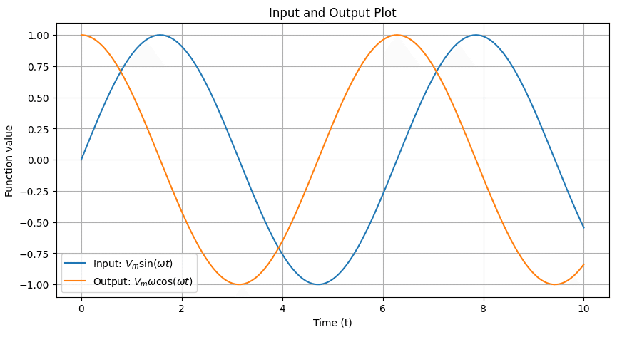
import numpy as np
import matplotlib.pyplot as plt

# Define symbols
t = np.linspace(0, 10, 1000)  # Divide time range into 1000 points from 0 to 10

# Define parameters
Vm = 1  # Placeholder value
omega = 1  # Placeholder value

# Calculate input function
input_function = Vm * np.sin(omega * t)

# Calculate output function
output_function = Vm * omega * np.cos(omega * t)

# Plot input and output
plt.figure(figsize=(10, 5))
plt.plot(t, input_function, label='Input: $V_m \sin(\omega t)$')
plt.plot(t, output_function, label='Output: $V_m \omega \cos(\omega t)$')
plt.xlabel('Time (t)')
plt.ylabel('Function value')
plt.title('Input and Output Plot')
plt.legend()
plt.grid(True)
plt.show()
import numpy as np
import matplotlib.pyplot as plt
from scipy import signal

# 与えられた伝達関数のパラメータ
a = 1.0
b = 100.0
f = 1000000.0

# 伝達関数の分子と分母の係数
numerator = [a]
denominator = [1.0, -(a*f), 0.0]

# 伝達関数の作成
system = signal.TransferFunction(numerator, denominator)

# ボード線図の計算
w, mag, phase = signal.bode(system)

# プロット
plt.figure()
plt.semilogx(w, mag)    # ゲインのボード線図
plt.grid(True)
plt.xlabel('Frequency [rad/s]')
plt.ylabel('Gain [dB]')
plt.title('Bode Plot (Magnitude)')
plt.figure()
plt.semilogx(w, phase)  # 位相のボード線図
plt.grid(True)
plt.xlabel('Frequency [rad/s]')
plt.ylabel('Phase [deg]')
plt.title('Bode Plot (Phase)')
plt.show()
def calculate_f(A, B, C, D):
    f = 1 / (1/A + 1/B + 1/C + 1/D)
    return f

# 与えられた値
A = 2
B = 3
C = 4
D = 5

# fの計算
result = calculate_f(A, B, C, D)
print("fの値は:", result)
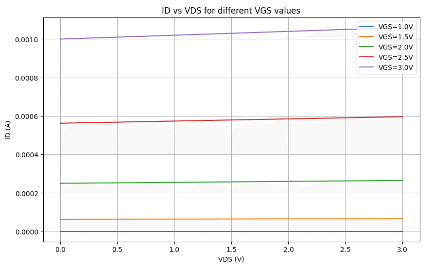
import numpy as np
import matplotlib.pyplot as plt
# MOSFET parameters
mu_Cox = 50e-6 # Mobility and oxide capacitance product (A/V^2)
W = 10e-6 # Width of the MOSFET (m)
L = 1e-6 # Length of the MOSFET (m)
Vth = 1.0 # Threshold voltage (V)
lambda_ = 0.02 # Channel-length modulation parameter (1/V)
# Function to calculate ID
def calculate_ID(VGS, VDS):
return (1/2) * mu_Cox * (W/L) * (VGS - Vth)**2 * (1 + lambda_ * VDS)
# VGS and VDS ranges
VGS_range = np.linspace(0, 3, 100) # Gate-source voltage range (V)
VDS_range = np.linspace(0, 3, 100) # Drain-source voltage range (V)
# Calculate ID for VGS-VDS graph
ID_VDS = np.array([[calculate_ID(VGS, VDS) for VDS in VDS_range] for VGS in VGS_range])
# Plot ID vs VDS for different VGS values
plt.figure(figsize=(10, 6))
for i, VGS in enumerate(np.linspace(1, 3, 5)):
plt.plot(VDS_range, calculate_ID(VGS, VDS_range), label=f'VGS={VGS:.1f}V')
plt.xlabel('VDS (V)')
plt.ylabel('ID (A)')
plt.title('ID vs VDS for different VGS values')
plt.legend()
plt.grid(True)
plt.show()
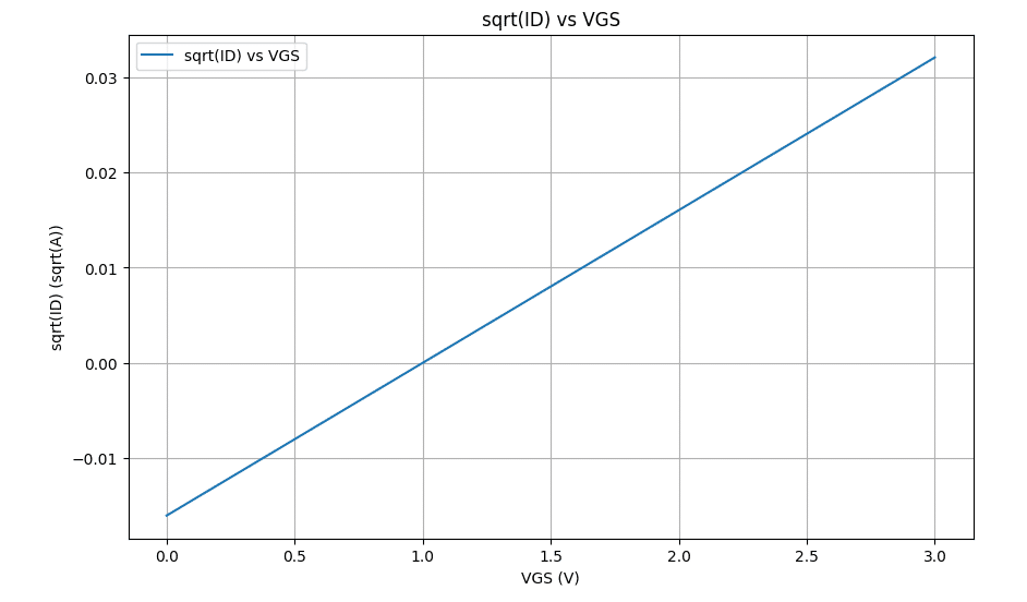
# Calculate sqrt(ID) for sqrt(ID) vs VGS graph
sqrt_ID_VGS = np.sqrt((1/2) * mu_Cox * (W/L)) * (VGS_range - Vth) * np.sqrt(1 + lambda_ * VDS_range.mean())
# Plot sqrt(ID) vs VGS
plt.figure(figsize=(10, 6))
plt.plot(VGS_range, sqrt_ID_VGS, label='sqrt(ID) vs VGS')
plt.xlabel('VGS (V)')
plt.ylabel('sqrt(ID) (sqrt(A))')
plt.title('sqrt(ID) vs VGS')
plt.legend()
plt.grid(True)
plt.show()
import math

# 定数の定義
μ = 0.02  # 遷移率 (example value in A/V^2)
Cox = 2.3e-3  # 酸化膜容量 (example value in F/m^2)
W = 1e-4  # チャンネル幅 (example value in m)
L = 1e-6  # チャンネル長 (example value in m)
λ = 0.02  # チャンネル長変調係数 (example value in V^-1)
Vth = 1.0  # 閾値電圧 (example value in V)

# 入力変数
ID = 1e-3  # ドレイン電流 (example value in A)
VGS = 2.0  # ゲート-ソース電圧 (example value in V)

# 小信号伝達コンダクタンス gm の計算
gm = math.sqrt(2 * μ * Cox * (W / L) * ID)

# 出力抵抗 ro の計算
ro = 1 / (0.5 * μ * Cox * (W / L) * λ * (VGS - Vth)**2)

# 結果の表示
print(f"小信号伝達コンダクタンス gm: {gm:.2e} S")
print(f"出力抵抗 ro: {ro:.2e} Ω")
import numpy as np
import matplotlib.pyplot as plt
from scipy.fft import fft

# Define the sampling frequency
Fs = 1024

# Create the time vector
t = np.arange(0, 1, 1/Fs)

# Create the time-domain signal
y = np.sin(2 * np.pi * 107 * t) + 0.6 * np.random.randn(len(t))

# Compute the FFT
Y = fft(y)

# Normalize the magnitude squared by the length
Py = (np.abs(Y) / len(Y)) ** 2

# Compute the power spectrum
Pyy = 10 * np.log10(Py)

# Create the frequency vector
f = Fs * np.arange(len(Y)) / len(Y)

# Plot the input waveform, time-domain signal, and the power spectrum
plt.figure()

plt.subplot(3, 1, 1)
plt.plot(t, np.sin(2 * np.pi * 107 * t))
plt.xlabel('Time (s)')
plt.ylabel('Amplitude')
plt.title('Input Waveform')

plt.subplot(3, 1, 2)
plt.plot(t, y)
plt.xlabel('Time (s)')
plt.ylabel('Amplitude')
plt.title('Noisy Time-Domain Signal')

plt.subplot(3, 1, 3)
plt.plot(f, Pyy)
plt.xlim([0, Fs / 2])
plt.xlabel('Frequency (Hz)')
plt.ylabel('Power (dB)')
plt.title('Power Spectrum')

plt.tight_layout()
plt.show()

import numpy as np
import matplotlib.pyplot as plt
from scipy import signal

# Define the parameters
A1 = 100  # Replace with the actual value
A2 = 10000  # Replace with the actual value
a = 10   # Replace with the actual value
b = 1000   # Replace with the actual value

# Define the transfer function G(s) = -A1*A2 / ((1 + s/a)(1 + s/b))
numerator = [-A1 * A2]
denominator = [1, (a + b), a * b]

# Create the transfer function
system = signal.TransferFunction(numerator, denominator)

# Define frequency range for Bode plot
omega = np.logspace(-2, 2, 500)

# Calculate Bode plot
w, mag, phase = signal.bode(system, w=omega)

# Plot magnitude
plt.figure()
plt.semilogx(w, mag)
plt.title('Bode Plot - Magnitude')
plt.xlabel('Frequency [rad/s]')
plt.ylabel('Magnitude [dB]')
plt.grid(True)

# Plot phase
plt.figure()
plt.semilogx(w, phase)
plt.title('Bode Plot - Phase')
plt.xlabel('Frequency [rad/s]')
plt.ylabel('Phase [degrees]')
plt.grid(True)

# Show plots
plt.show()
import math

# 定数
μ = 600  # モビリティ(μ)
Cox = 3.45e-6  # ゲート酸化膜容量(Cox)
VA = 50  # マクスウェルの等価時間定数(VA)

# 入力値
IDS = 1e-3  # Drain to Source電流(IDS)
Vov = 2  # オーバードライブ電圧(Vov)
VDS = 5  # Drain to Source電圧(VDS)
gm = 0.01  # トランジスタのトランスコンダクタンス(gm)
ID = 0.5e-3  # Drain電流(ID)
I5 = 2e-3  # Drain電流(I5)

# 式1の計算
WL_1 = 2 * IDS / (μ * Cox * (Vov**2) * (1 + VDS/VA))

# 式2の計算
WL_2 = (gm**2) / (2 * μ * Cox * ID)

# 式3の計算
WL_3 = (2 * I5) / (μ * Cox * (VDS**2))

# 式4の計算
I6 = gm / (2 * μ * Cox * WL_1)

print("式1の計算結果 (W/L) =", WL_1)
print("式2の計算結果 (W/L) =", WL_2)
print("式3の計算結果 (W/L) =", WL_3)
print("式4の計算結果 (I6) =", I6)
import math

# Given parameters
μ = 600  # Mobility (cm^2/Vs)
Cox = 1.6e-6  # Oxide capacitance per unit area (F/cm^2)
W_L = 10  # Width-to-length ratio
VGS = 1.5  # Gate-source voltage (V)
Vth = 0.7  # Threshold voltage (V)
IDS = 2e-3  # Drain current (A)

# Calculating gm1
gm1 = μ * Cox * (W_L) * (VGS - Vth)

# Calculating gm2
gm2 = 2 * math.sqrt(μ * Cox * 0.5 * (W_L) * IDS)

# Calculating gm3
gm3 = 2 * IDS / (VGS - Vth)

print("gm1 =", gm1)
print("gm2 =", gm2)
print("gm3 =", gm3)
def gd1(W, L, VGS, Vth, VA, Cox, μ):
    return (μ * Cox * (1/2)) * (W/L) * ((VGS - Vth)**2) / VA

def gd2(IDS, VDS, VA):
    return IDS / ((1 + VDS/VA) * VA)

def gd3(ID, VDS, VA):
    return ID / (VA + VDS)

# 値を設定
W = 1.0  # チャネル幅 (W)
L = 1.0  # チャネル長 (L)
VGS = 3.0  # ゲート-ソース電圧 (VGS)
Vth = 1.0  # 閾値電圧 (Vth)
VA = 10.0  # Early電圧 (VA)
Cox = 1.0  # ゲート容量 (Cox)
μ = 1.0  # 移動度 (μ)
IDS = 2.0  # ドレイン-ソース電流 (IDS)
ID = 1.0  # ドレイン電流 (ID)
VDS = 5.0  # ドレイン-ソース電圧 (VDS)

# 関数を呼び出して出力コンダクタンスを計算
print("gd1:", gd1(W, L, VGS, Vth, VA, Cox, μ))
print("gd2:", gd2(IDS, VDS, VA))
print("gd3:", gd3(ID, VDS, VA))
def calculate_gm1(mu, Cox, W_over_L, VGS, Vth):
    gm1 = mu * Cox * W_over_L * (VGS - Vth)
    return gm1

def calculate_gm2(IDS, VGS, Vth):
    gm2 = (2 * IDS) / (VGS - Vth)
    return gm2

# 定数と入力値の定義
mu = 1000 # μ
Cox = 1e-6 # Cox (F/cm^2)
W_over_L = 10 # W/L
VGS = 2.5 # VGS (V)
Vth = 0.5 # Vth (V)
IDS = 0.001 # IDS (A)

# gm1とgm2の計算
gm1 = calculate_gm1(mu, Cox, W_over_L, VGS, Vth)
gm2 = calculate_gm2(IDS, VGS, Vth)

print("gm1:", gm1)
print("gm2:", gm2)
import math

# 定数の値
IDS = 0.1  # drain-source電流 (A)
μ = 600  # チャネルモビリティ (cm^2/Vs)
Cox = 1.5e-6  # ゲート酸化物キャパシタンス (F/cm^2)
W_over_L = 10  # 幅対長さ比
Vth = 1  # 閾値電圧 (V)
VA = 5  # Early電圧 (V)
VDS = 2  # drain-source電圧 (V)

# VGSを計算する式
VGS = math.sqrt(2 * IDS / (μ * Cox * (W_over_L) * (1 + VDS / VA))) + Vth

# gdを計算する式
gd = IDS / (VA + VDS)

print("VGS:", VGS)
print("gd:", gd)
def calculate_mu_cox(WL, VDS, VA, gm):
    mu_cox = gm / (WL * (1 + VDS / VA))
    return mu_cox

WL = 10
VDS = 2
VA = 10
gm = 0.1

mu_cox = calculate_mu_cox(WL, VDS, VA, gm)
print("μCox =", mu_cox)
import numpy as np
import matplotlib.pyplot as plt

# 係数の値を設定
A = 10
B = 1000
C = 1000000

# 周波数の範囲を設定
omega = np.logspace(0, 6, 1000)

# 伝達関数の振幅と位相を計算
magnitude = 20 * np.log10(B / np.sqrt((C - omega**2)**2 + (A * omega)**2))
phase = np.arctan2(-A * omega, (C - omega**2)) * 180 / np.pi

# プロット
plt.figure()
plt.subplot(2, 1, 1)
plt.semilogx(omega, magnitude)
plt.title('Bode Plot')
plt.ylabel('Magnitude [dB]')

plt.subplot(2, 1, 2)
plt.semilogx(omega, phase)
plt.xlabel('Frequency [rad/s]')
plt.ylabel('Phase [deg]')
plt.show()
import sympy as sp
import numpy as np
import matplotlib.pyplot as plt
from scipy import signal

# Parameters
a, b, z = sp.symbols('a b z')

# Transfer function components
numerator = a + z**(-1)
denominator = 1 - a*b - b*z**(-1)

# Simplify the transfer function
transfer_function = numerator / denominator
transfer_function_simplified = sp.simplify(transfer_function)
print(f"Simplified Transfer Function: {transfer_function_simplified}")

# Substitute a and b with specific values (example values)
a_value = 1  # Example value for a
b_value = 2  # Example value for b

# Create the transfer function for specific values of a and b
num = [a_value, 1]
den = [1, -a_value*b_value, -b_value]

# Create the transfer function object
system = signal.TransferFunction(num, den, dt=True)

# Generate the Bode plot
w, mag, phase = signal.dbode(system)

# Plot the magnitude and phase
plt.figure()
plt.subplot(2, 1, 1)
plt.semilogx(w, mag)
plt.title('Bode plot')
plt.ylabel('Magnitude (dB)')

plt.subplot(2, 1, 2)
plt.semilogx(w, phase)
plt.xlabel('Frequency [rad/sample]')
plt.ylabel('Phase (degrees)')
plt.show()
def voltage_gain(gm, gmb, RL, RS):
    # Source-grounded voltage gain
    Av_source_grounded = -gm * RL

    # Drain-grounded voltage gain
    Av_drain_grounded = gm / (gm + gmb)

    # Gate-grounded voltage gain
    Av_gate_grounded = (gm + gmb) * RL

    # Load resistance RL drain-grounded voltage gain
    Av_RL_drain_grounded = -gm * RL / (1 + gm * RS)

    # Source-grounded with a resistance between source and ground voltage gain
    Av_source_resistance_grounded = gm / (1 + gm * RS)

    return {
        'Av_source_grounded': Av_source_grounded,
        'Av_drain_grounded': Av_drain_grounded,
        'Av_gate_grounded': Av_gate_grounded,
        'Av_RL_drain_grounded': Av_RL_drain_grounded,
        'Av_source_resistance_grounded': Av_source_resistance_grounded
    }

# Example parameters
gm = 1e-3  # transconductance in Siemens
gmb = 1e-4 # body transconductance in Siemens
RL = 1e3   # load resistance in Ohms
RS = 1e2   # source resistance in Ohms

# Calculate voltage gains
voltage_gains = voltage_gain(gm, gmb, RL, RS)

# Print results
for key, value in voltage_gains.items():
    print(f"{key}: {value:.4f}")
import numpy as np
import matplotlib.pyplot as plt

# 定数
IS = 1e-12  # 飽和電流 (A)
q = 1.60217662e-19  # 電子の電荷 (C)
k = 1.38064852e-23  # ボルツマン定数 (J/K)
T = 300  # 絶対温度 (K)

# 電圧範囲
V = np.linspace(0, 0.7, 500)  # 0Vから0.7Vまで500ポイント

# 電流を計算
I = IS * (np.exp(q * V / (k * T)) - 1)

# プロット
plt.figure(figsize=(8, 6))
plt.plot(V, I, label='I-V Curve')
plt.xlabel('Voltage (V)')
plt.ylabel('Current (A)')
plt.title('I-V Characteristics')
plt.grid(True)
plt.legend()
plt.show()
import numpy as np
import matplotlib.pyplot as plt

# 定数を定義
V = 10  # 電圧の例
Rout = 5  # Routの例

# P(Rin)の関数を定義
def P(Rin, V, Rout):
    return (Rin * V**2) / (Rin + Rout)**2

# Rinの範囲を設定
Rin_values = np.linspace(0.1, 100, 500)  # 0.1から100までの500ポイント

# P(Rin)の値を計算
P_values = P(Rin_values, V, Rout)

# プロットを作成
plt.figure(figsize=(10, 6))
plt.plot(Rin_values, P_values, label='P(Rin)')
plt.xlabel('Rin')
plt.ylabel('P(Rin)')
plt.title('P(Rin) vs Rin')
plt.legend()
plt.grid(True)
plt.show()
import numpy as np
import matplotlib.pyplot as plt

# 定数の設定
IS = 1e-12  # サンプルの飽和電流(単位: A)
thermal_voltage = 26e-3  # 熱電圧(単位: V)

# VBEの範囲を設定
VBE = np.linspace(0, 0.8, 500)

# ICの計算
IC = IS * np.exp(VBE / thermal_voltage)

# プロット
plt.figure(figsize=(10, 6))
plt.plot(VBE, IC)
plt.xlabel('VBE (V)')
plt.ylabel('IC (A)')
plt.title('IC vs VBE')
plt.grid(True)
plt.show()
import math

def calculate_parameters(n, VFS, T):
    # 2^n レベルの計算
    levels = 2 ** n

    # フルスケール(FS)周波数の計算
    FS = 1 / T

    # 1 LSBの計算
    LSB = VFS / (levels - 1)

    # 量子化ノイズ電圧の計算
    quantization_noise_voltage = LSB / math.sqrt(12)

    # SNRの計算
    SNR = 6.02 * n + 1.76

    # ENOBの計算
    ENOB = (SNR - 1.76) / 6.02

    return {
        'レベル数': levels,
        'フルスケール周波数': FS,
        '1 LSB': LSB,
        '量子化ノイズ電圧': quantization_noise_voltage,
        'SNR': SNR,
        'ENOB': ENOB
    }

# 使用例
n = 8  # ビット数
VFS = 5.0  # フルスケール電圧(ボルト単位)
T = 1e-6  # 周期(秒単位)

parameters = calculate_parameters(n, VFS, T)
for key, value in parameters.items():
    print(f"{key}: {value}")
import numpy as np
import matplotlib.pyplot as plt

# パラメータ設定
n = 1024  # データ数
dt = 0.01  # サンプリング間隔 [sec]
t = np.arange(n) * dt  # 時間ベクトル
Fin = 10  # 入力信号の周波数 [Hz]
Fs = 1 / dt  # サンプリング周波数 [Hz]

# 方形波生成
y = np.sign(np.sin(2 * np.pi * Fin * t))

# 方形波のプロット
plt.figure()
plt.plot(t, y)
plt.xlabel('Time [sec]')
plt.ylabel('Magnitude')
plt.xlim([0, 1])
plt.title('Square Wave')
plt.show()

# FFTの実行
Y = np.fft.fft(y)
frequencies = np.fft.fftfreq(n, dt)

# パワースペクトルの計算
power = np.abs(Y)**2 / n

# FFTのプロット
plt.figure()
plt.plot(frequencies[:n // 2], power[:n // 2])  # 正の周波数成分のみプロット
plt.xlabel('Frequency [Hz]')
plt.ylabel('Power')
plt.title('Power Spectrum')
plt.xlim([0, Fs/2])  # Nyquist周波数までプロット
plt.show()

# SNRの計算
signal_power = np.sum(power[np.abs(frequencies - Fin) < (Fs / n)])
noise_power = np.sum(power) - signal_power
SNR = 10 * np.log10(signal_power / noise_power)

print(f'Signal Power: {signal_power:.2f}')
print(f'Noise Power: {noise_power:.2f}')
print(f'SNR: {SNR:.2f} dB')
import numpy as np
import matplotlib.pyplot as plt

# パラメータの設定
Fs = 1000  # サンプリング周波数 (Hz)
T = 1 / Fs  # サンプリング周期
t = np.arange(0, 1, T)  # 時間軸 (1秒間)
f = 5  # 方形波の周波数 (Hz)

# 方形波の生成
square_wave = 0.5 * (1 + np.sign(np.sin(2 * np.pi * f * t)))

# ノイズを追加
noise = np.random.normal(0, 0.1, len(t))
noisy_signal = square_wave + noise

# プロット
plt.figure(figsize=(10, 4))
plt.plot(t, noisy_signal, label='Noisy Square Wave')
plt.title('Noisy Square Wave Signal')
plt.xlabel('Time [s]')
plt.ylabel('Amplitude')
plt.legend()
plt.grid(True)
plt.show()

# FFTの計算
N = len(noisy_signal)
fft_output = np.fft.fft(noisy_signal)
fft_freqs = np.fft.fftfreq(N, T)

# パワースペクトルの計算
power_spectrum = np.abs(fft_output) ** 2

# プロット (パワースペクトル)
plt.figure(figsize=(10, 4))
plt.plot(fft_freqs[:N // 2], power_spectrum[:N // 2])
plt.title('Power Spectrum')
plt.xlabel('Frequency [Hz]')
plt.ylabel('Power')
plt.grid(True)
plt.show()

# SNRの計算
signal_power = np.sum(power_spectrum[(fft_freqs >= 0) & (fft_freqs < 2 * f)])
noise_power = np.sum(power_spectrum) - signal_power
SNR = 10 * np.log10(signal_power / noise_power)

print(f'Signal Power: {signal_power}')
print(f'Noise Power: {noise_power}')
print(f'SNR: {SNR:.2f} dB')
import numpy as np
import matplotlib.pyplot as plt

# パラメータ設定
N =  1024  # Nは2のべき乗
M = 101  # Mは素数
fin_fs = M / N  # fin / fs の比
fs = 1.0  # サンプリング周波数 (正規化のために1とする)
fin = fin_fs * fs  # 入力周波数

# 方形波の生成
t = np.arange(N) / fs
input_signal = np.sign(np.sin(2 * np.pi * fin * t))

# 8ビット量子化
quantized_signal = np.round(((input_signal + 1) / 2) * 255) / 255 * 2 - 1

# FFT計算
fft_result = np.fft.fft(quantized_signal)
fft_freqs = np.fft.fftfreq(N, 1 / fs)
power_spectrum = np.abs(fft_result) ** 2 / N

# 方形波の入力プロット
plt.figure(figsize=(10, 6))
plt.subplot(2, 1, 1)
plt.plot(t, input_signal)
plt.xlabel('Time (s)')
plt.ylabel('Amplitude')
plt.title('Input Square Wave')
plt.grid(True)

# ADC出力のプロット
plt.subplot(2, 1, 2)
plt.plot(t, quantized_signal)
plt.xlabel('Time (s)')
plt.ylabel('Amplitude')
plt.title('Quantized Signal (ADC Output)')
plt.grid(True)

plt.tight_layout()
plt.show()

# パワースペクトル表示
plt.figure(figsize=(10, 6))
plt.plot(fft_freqs[:N//2], 10 * np.log10(power_spectrum[:N//2]))
plt.xlabel('Frequency (Hz)')
plt.ylabel('Power Spectrum (dB)')
plt.title('Power Spectrum of ADC Output')
plt.grid(True)
plt.show()

# SNR計算
signal_power = np.sum(power_spectrum[(fft_freqs >= fin - fin_fs/2) & (fft_freqs <= fin + fin_fs/2)])
noise_power = np.sum(power_spectrum[(fft_freqs < fin - fin_fs/2) | (fft_freqs > fin + fin_fs/2)])
SNR = 10 * np.log10(signal_power / noise_power)

print(f'Signal Power: {signal_power:.2f}')
print(f'Noise Power: {noise_power:.2f}')
print(f'SNR: {SNR:.2f} dB')
import numpy as np
import matplotlib.pyplot as plt

# Parameters
fs = 1000  # Sampling frequency
T = 1  # seconds
f_signal = 50  # Signal frequency
amplitude_signal = 1  # Signal amplitude
amplitude_noise = 0.1  # Noise amplitude

# Time array
t = np.linspace(0, T, int(fs*T), endpoint=False)

# Generate a sine wave signal
signal = amplitude_signal * np.sin(2 * np.pi * f_signal * t)

# Add some random noise
noise = amplitude_noise * np.random.randn(len(t))
adc_output = signal + noise

# Plot ADC Output (Digital Code)
plt.figure(figsize=(12, 6))

plt.subplot(2, 1, 1)
plt.plot(t, adc_output, label='ADC Output')
plt.plot(t, signal, 'r', label='Original Signal')
plt.legend()
plt.title('ADC Output (Digital Code)')
plt.xlabel('Time [s]')
plt.ylabel('Amplitude')

# Perform FFT
N = len(adc_output)
fft_result = np.fft.fft(adc_output)
fft_freq = np.fft.fftfreq(N, 1/fs)

# Power spectrum
power_spectrum = np.abs(fft_result)**2 / N

# Plot Power Spectrum
plt.subplot(2, 1, 2)
plt.plot(fft_freq[:N//2], 10 * np.log10(power_spectrum[:N//2]), 'r')
plt.title('Output Power Spectrum')
plt.xlabel('Frequency [Hz]')
plt.ylabel('Power [dB]')

plt.tight_layout()
plt.show()

# Signal and Noise Power
signal_power = np.sum(power_spectrum[(fft_freq >= f_signal-1) & (fft_freq <= f_signal+1)])
noise_power = np.sum(power_spectrum[(fft_freq < f_signal-1) | (fft_freq > f_signal+1)])

# Calculate SNR
SNR_dB = 10 * np.log10(signal_power / noise_power)
print(f"SNR[dB] = {SNR_dB:.2f} dB")
import numpy as np
import matplotlib.pyplot as plt
from scipy.fft import fft, fftfreq

# 定数の定義
fin = 10  # 周波数 10Hz
t = np.linspace(0, 0.1, 1000, endpoint=False)  # 時間 0~0.1秒
A = np.sin(2 * np.pi * fin * t)  # 正弦波生成

# デジタルコードに変換
A_511 = np.round((A + 1) * 255.5).astype(int)  # [0, 511]の範囲に変換
A_1023 = np.round((A + 1) * 511.5).astype(int)  # [0, 1023]の範囲に変換

# 波形のプロット
plt.figure(figsize=(12, 6))
plt.subplot(2, 1, 1)
plt.plot(t, A_511)
plt.title('Waveform [0-511]')
plt.xlabel('Time [s]')
plt.ylabel('Amplitude')

plt.subplot(2, 1, 2)
plt.plot(t, A_1023)
plt.title('Waveform [0-1023]')
plt.xlabel('Time [s]')
plt.ylabel('Amplitude')

plt.tight_layout()
plt.show()

# FFTの実行
N = len(t)
A_511_fft = fft(A_511)
A_1023_fft = fft(A_1023)
freqs = fftfreq(N, t[1] - t[0])

# パワースペクトルの計算
power_511 = np.abs(A_511_fft)**2
power_1023 = np.abs(A_1023_fft)**2

# パワースペクトルのプロット
plt.figure(figsize=(12, 6))
plt.subplot(2, 1, 1)
plt.plot(freqs[:N // 2], power_511[:N // 2])
plt.title('Power Spectrum [0-511]')
plt.xlabel('Frequency [Hz]')
plt.ylabel('Power')

plt.subplot(2, 1, 2)
plt.plot(freqs[:N // 2], power_1023[:N // 2])
plt.title('Power Spectrum [0-1023]')
plt.xlabel('Frequency [Hz]')
plt.ylabel('Power')

plt.tight_layout()
plt.show()

# SN比の計算
signal_power_511 = power_511[fin * N // 1000]
noise_power_511 = np.sum(power_511) - signal_power_511
snr_511 = 10 * np.log10(signal_power_511 / noise_power_511)

signal_power_1023 = power_1023[fin * N // 1000]
noise_power_1023 = np.sum(power_1023) - signal_power_1023
snr_1023 = 10 * np.log10(signal_power_1023 / noise_power_1023)

print(f'SNR for [0-511] digital code: {snr_511:.2f} dB')
print(f'SNR for [0-1023] digital code: {snr_1023:.2f} dB')
def source_common_amplifier_gain(gm, RD, RL):
    """
    ソース接地増幅回路の増幅率を計算する。

    :param gm: トランスコンダクタンス (A/V)
    :param RD: ドレイン抵抗 (Ω)
    :param RL: 負荷抵抗 (Ω)
    :return: 増幅率
    """
    gain = gm * (RD * RL) / (RD + RL)
    return gain

def drain_common_amplifier_gain(gm, RS):
    """
    ドレイン接地増幅回路の増幅率を計算する。

    :param gm: トランスコンダクタンス (A/V)
    :param RS: ソース抵抗 (Ω)
    :return: 増幅率
    """
    gain = 1 - 1 / (1 + RS * gm)
    return gain

# 例としてのパラメータ設定
gm = 2e-3  # トランスコンダクタンス (A/V)
RD = 1e3  # ドレイン抵抗 (Ω)
RL = 1e3  # 負荷抵抗 (Ω)
RS = 500  # ソース抵抗 (Ω)

# ソース接地増幅回路の増幅率を計算
source_gain = source_common_amplifier_gain(gm, RD, RL)
print(f"ソース接地増幅回路の増幅率: {source_gain}")

# ドレイン接地増幅回路の増幅率を計算
drain_gain = drain_common_amplifier_gain(gm, RS)
print(f"ドレイン接地増幅回路の増幅率: {drain_gain}")
import numpy as np
import matplotlib.pyplot as plt

# Definitions
t = np.linspace(0, 1, 1000)  # Time
f_info = 5  # Information signal frequency (Hz)
f_carrier = 100  # Carrier wave frequency (Hz)
A = 1  # Carrier amplitude
m = 0.5  # Modulation index

# Information signal
info_signal = np.sin(2 * np.pi * f_info * t)

# Carrier wave
carrier_signal = A * np.cos(2 * np.pi * f_carrier * t)

# Modulated signal
modulated_signal = (A + m * info_signal) * np.cos(2 * np.pi * f_carrier * t)

# Plotting
plt.figure(figsize=(15, 10))

# Information signal plot
plt.subplot(3, 1, 1)
plt.plot(t, info_signal)
plt.title('Information Signal')
plt.xlabel('Time (s)')
plt.ylabel('Amplitude')

# Carrier wave plot
plt.subplot(3, 1, 2)
plt.plot(t, carrier_signal)
plt.title('Carrier Wave')
plt.xlabel('Time (s)')
plt.ylabel('Amplitude')

# Modulated signal plot
plt.subplot(3, 1, 3)
plt.plot(t, modulated_signal)
plt.title('Modulated Signal')
plt.xlabel('Time (s)')
plt.ylabel('Amplitude')

plt.tight_layout()
plt.show()
import numpy as np
import matplotlib.pyplot as plt

# Parameters
fs = 1000  # Sampling frequency
t = np.arange(0, 1, 1/fs)  # Time axis

# Information signal (example: sine wave)
f_m = 5  # Frequency of the information signal
A_m = 1  # Amplitude of the information signal
m = A_m * np.sin(2 * np.pi * f_m * t)

# Carrier wave
f_c = 100  # Frequency of the carrier wave
A_c = 1  # Amplitude of the carrier wave
c = A_c * np.cos(2 * np.pi * f_c * t)

# FM modulation
kf = 2 * np.pi * 10  # Frequency sensitivity
s = A_c * np.cos(2 * np.pi * f_c * t + kf * np.cumsum(m) / fs)

# Plotting
plt.figure(figsize=(12, 8))

plt.subplot(3, 1, 1)
plt.plot(t, m)
plt.title('Information Signal')
plt.xlabel('Time [s]')
plt.ylabel('Amplitude')

plt.subplot(3, 1, 2)
plt.plot(t, c)
plt.title('Carrier Wave')
plt.xlabel('Time [s]')
plt.ylabel('Amplitude')

plt.subplot(3, 1, 3)
plt.plot(t, s)
plt.title('FM Modulated Signal')
plt.xlabel('Time [s]')
plt.ylabel('Amplitude')

plt.tight_layout()
plt.show()
import numpy as np
import matplotlib.pyplot as plt
from scipy.fft import fft

# パラメータ設定
fin = 10  # 周波数10Hz
t = np.linspace(0, 0.1, 1000)  # 0〜0.1秒の時間範囲で1000点
A = np.sin(2 * np.pi * fin * t)  # 正弦波の生成

# 正弦波のプロット
plt.figure(figsize=(12, 6))
plt.subplot(2, 2, 1)
plt.plot(t, A)
plt.title('Analog Signal')
plt.xlabel('Time [s]')
plt.ylabel('Amplitude')

# AD変換関数
def adc_conversion(signal, bits):
    VFS = 1.0  # フルスケールの振幅 (ここでは正規化して1とする)
    q = VFS / (2**bits - 1)
    digital_code = np.round((signal + 1) / 2 * (2**bits - 1)).astype(int)  # 正規化してから量子化
    return digital_code

# 9ビットと10ビットのAD変換
digital_code_9bit = adc_conversion(A, 9)
digital_code_10bit = adc_conversion(A, 10)

# デジタル信号のプロット
plt.subplot(2, 2, 2)
plt.plot(t, digital_code_9bit)
plt.title('Digital Signal (9-bit)')
plt.xlabel('Time [s]')
plt.ylabel('Digital Code')

plt.subplot(2, 2, 3)
plt.plot(t, digital_code_10bit)
plt.title('Digital Signal (10-bit)')
plt.xlabel('Time [s]')
plt.ylabel('Digital Code')

# FFTの実行
fft_9bit = fft(digital_code_9bit)
fft_10bit = fft(digital_code_10bit)

# パワースペクトルの計算
power_spectrum_9bit = np.abs(fft_9bit)**2
power_spectrum_10bit = np.abs(fft_10bit)**2

# 周波数軸の生成
freqs = np.fft.fftfreq(len(t), d=t[1] - t[0])

# パワースペクトルのプロット
plt.subplot(2, 2, 4)
plt.plot(freqs[:len(freqs)//2], power_spectrum_9bit[:len(freqs)//2], label='9-bit')
plt.plot(freqs[:len(freqs)//2], power_spectrum_10bit[:len(freqs)//2], label='10-bit')
plt.title('Power Spectrum')
plt.xlabel('Frequency [Hz]')
plt.ylabel('Power')
plt.legend()

plt.tight_layout()
plt.show()

# SNRの計算関数
def calculate_snr(power_spectrum):
    signal_power = np.max(power_spectrum)
    noise_power = np.sum(power_spectrum) - signal_power
    snr = 10 * np.log10(signal_power / noise_power)
    return snr

# SN比の計算
snr_9bit = calculate_snr(power_spectrum_9bit)
snr_10bit = calculate_snr(power_spectrum_10bit)

print(f"SNR (9-bit): {snr_9bit:.2f} dB")
print(f"SNR (10-bit): {snr_10bit:.2f} dB")
この記事が気に入ったらサポートをしてみませんか?