Trying Data Science(9) : Cramming Linear Regression

This posting is a practice for Linear Regression. Let's suppose that a company is trying to decide whether to focus its efforts on mobile app experience or website. You should do like this.

Imports

---

import pandas as pd
import numpy as np
import matplotlib.pyplot as plt
import seaborn as sns
%matplotlib inline

Get/Check the Data 

---

customers = pd.read_csv("Ecommerce Customers")
customers.head()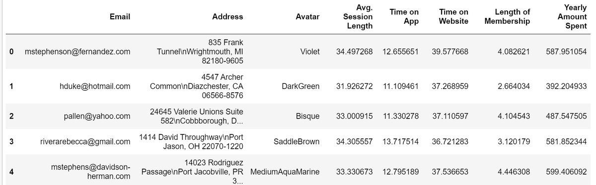

customers.describe()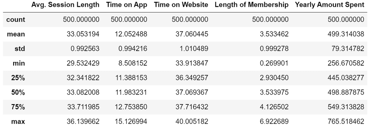

customers.info()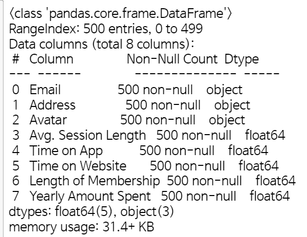

Exploratory Data Analysis

---

Use seaborn to create a jointplot to compare the Time on Website and Yearly Amount Spent columns. How about the correlation?

sns.set_palette("GnBu_d")
sns.set_style('whitegrid')

# More time on site, more money spent.
sns.jointplot(x='Time on Website',y='Yearly Amount Spent',data=customers)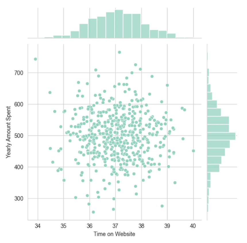

Time on Website / Amount Spent

sns.jointplot(x='Time on App',y='Yearly Amount Spent',data=customers)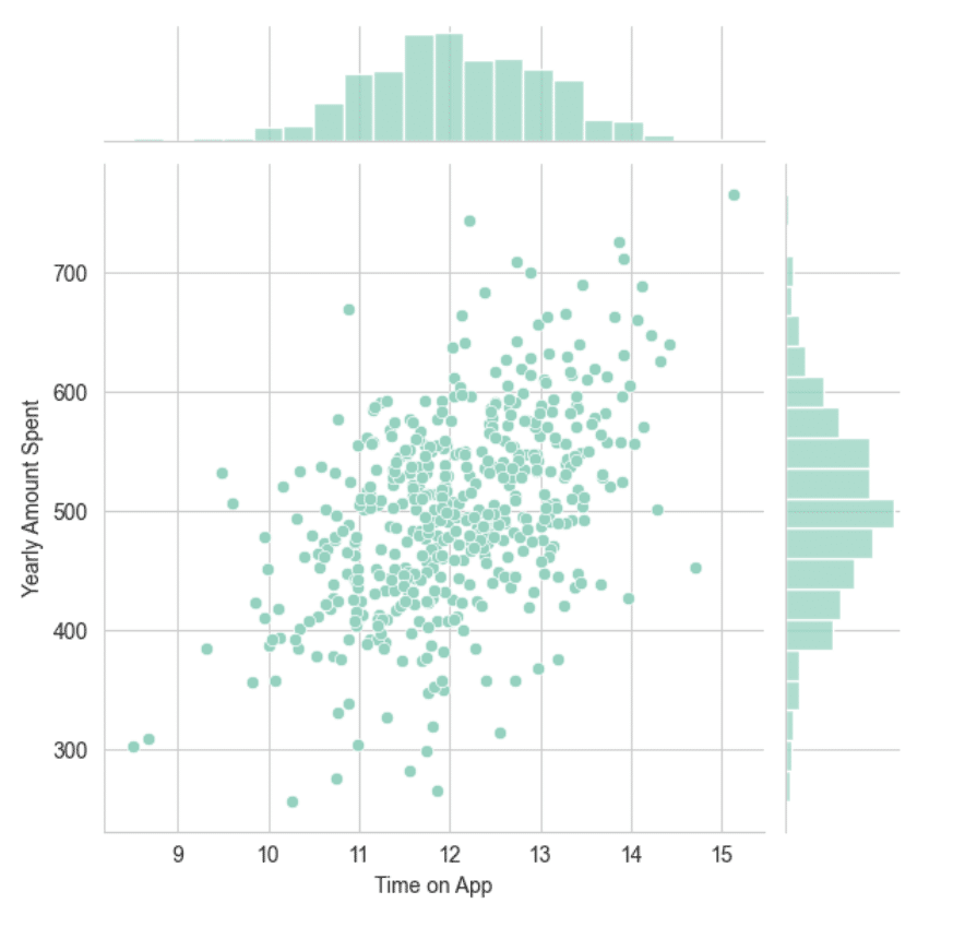

sns.pairplot(customers)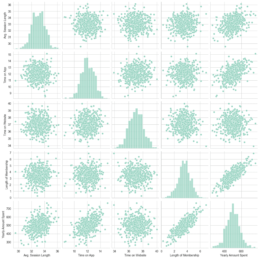

The most correlated feature with Yearly Amount Spent is Length of Membership.

A linear model plot of Yearly Amount Spent `. Length of Membership.

sns.lmplot(x='Length of Membership',y='Yearly Amount Spent',data=customers)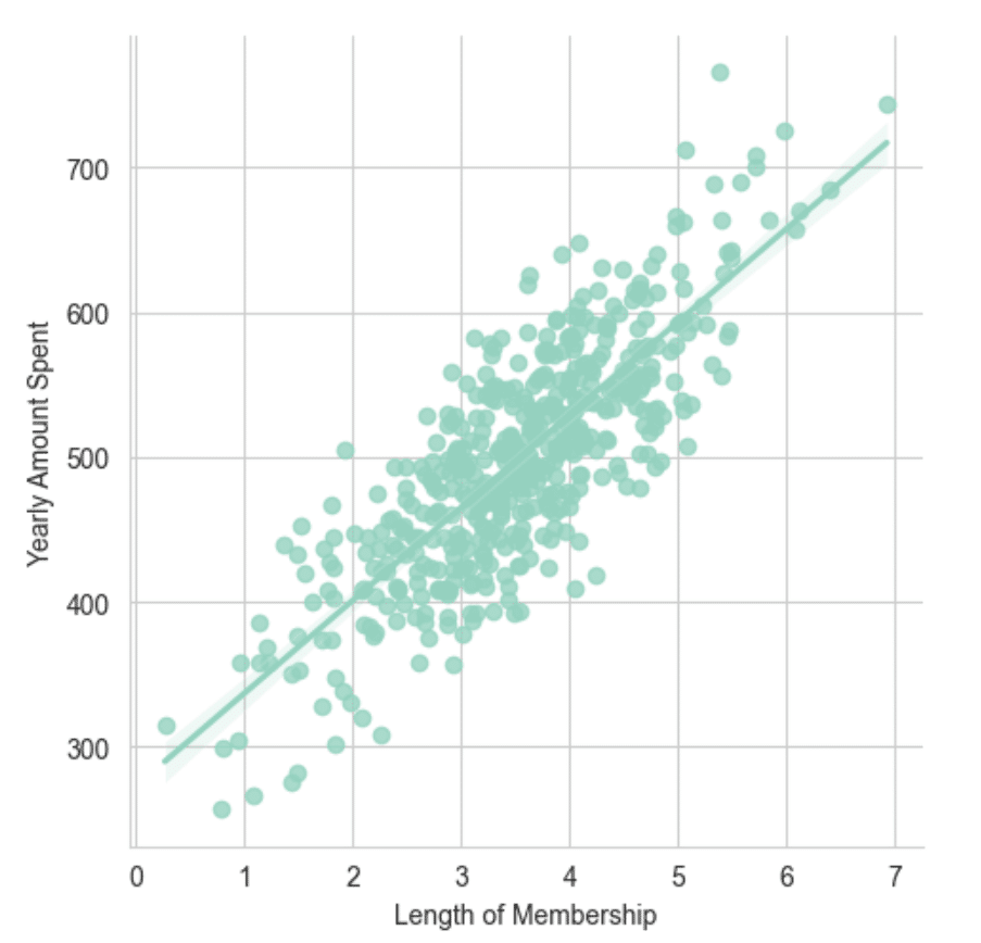

Training and Testing Data

---

Let's go ahead and split the data into training and testing sets.

Set a variable X equal to the numerical features of the customers and a variable y equal to the "Yearly Amount Spent" column.

y = customers['Yearly Amount Spent']
X = customers[['Avg. Session Length', 'Time on App','Time on Website', 'Length of Membership']]

from sklearn.model_selection import train_test_split
X_train, X_test, y_train, y_test = train_test_split(X, y, test_size=0.3, random_state=101)

Training the Model

---

Import LinearRegression from sklearn.linear_model

from sklearn.linear_model import LinearRegression

Create an instance of a LinearRegression() model named lm

lm = LinearRegression()

Train/fit lm on the training data.

lm.fit(X_train,y_train)

Print out the coefficients of the model

# The coefficients
print('Coefficients: \n', lm.coef_)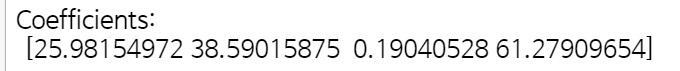

Predicting Test Data

---

Let's evaluate its performance by predicting off the test values.

Use lm.predict() to predict off the X_test set of the data.

predictions = lm.predict( X_test)

Create a scatterplot of the real test values versus the predicted values.

plt.scatter(y_test,predictions)
plt.xlabel('Y Test')
plt.ylabel('Predicted Y')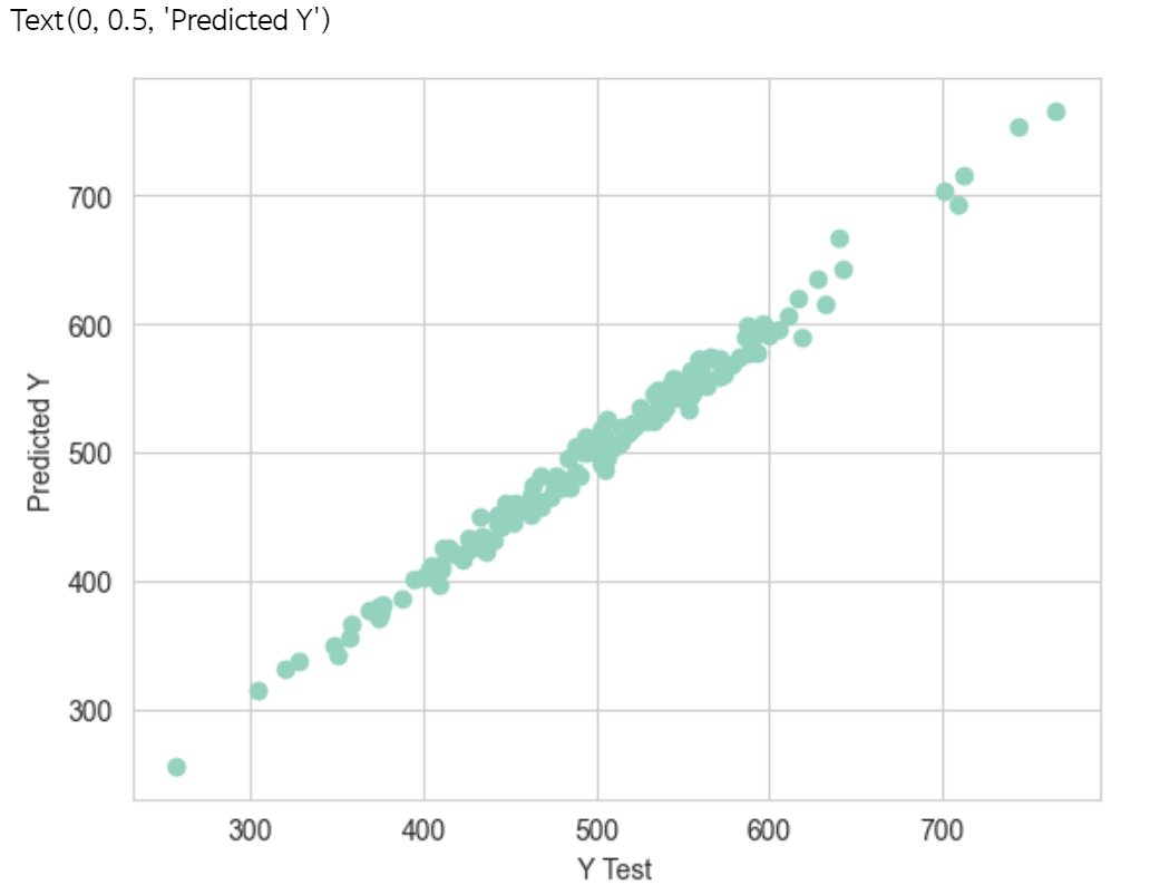

Evaluating the Model

---

Calculate the Mean Absolute Error, Mean Squared Error, and the Root Mean Squared Error.

from sklearn import metrics

print('MAE:', metrics.mean_absolute_error(y_test, predictions))
print('MSE:', metrics.mean_squared_error(y_test, predictions))
print('RMSE:', np.sqrt(metrics.mean_squared_error(y_test, predictions)))

Residuals

---

Let's quickly explore the residuals to make sure everything was okay with our data.

Plot a histogram of the residuals and make sure it looks normally distributed.

sns.distplot((y_test-predictions),bins=50);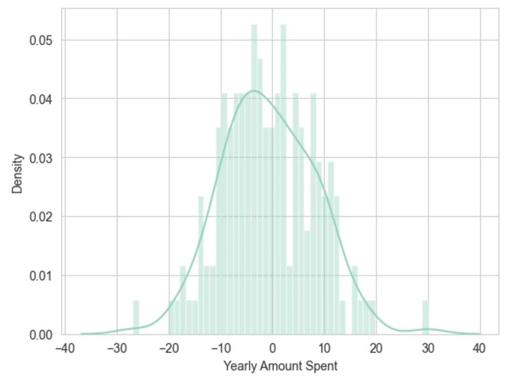

Conclusion

---

Do we focus our efforts on mobile app or website development? Or Maybe that doesn't really matter, because Membership Time is what is really important?

coeffecients = pd.DataFrame(lm.coef_,X.columns)
coeffecients.columns = ['Coeffecient']
coeffecients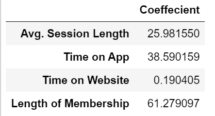

How can you interpret these coefficients? 

• Holding all other features fixed, a 1 unit increase in Avg. Session Length is associated with an increase of 25.98 total dollars spent.

• Holding all other features fixed, a 1 unit increase in Time on App is associated with an increase of 38.59 total dollars spent.

• Holding all other features fixed, a 1 unit increase in Time on Website is associated with an increase of 0.19 total dollars spent.

• Holding all other features fixed, a 1 unit increase in Length of Membership is associated with an increase of 61.27 total dollars spent.

So,

1.  Develop the Website to catch up to the performance of the mobile app

2.  Develop the app more since that is what is working better.

A answer depends on the other factors going on at the company.

ソンさん