逆関数法(Inverse transform sampling)

アルちゃん

2023年9月3日 07:46

まだ未検証。

参考

逆関数法

一様乱数から特定の確率分布に従う乱数をつくる。

累積分布関数(CDF)を求める: 確率変数$${X}$$が持つ確率密度関数(pdf)を$${f(x)}$$としたとき、その累積分布関数(CDF) $${F(x)}$$は以下の式で定義されます。 $${F(x) = P(X \leq x) = \int_{-\infty}^{x} f(t) dt}$$
一様乱数を生成する: 0と1の間の一様乱数Uを生成します。
CDFの逆関数を使用する: Fの逆関数$${F^{−1}(u)}$$を使用して、$${u = F(x)}$$を$${x}$$に関して解きます。
サンプルを得る: $${F^{−1}(U)}$$の値は、所望の確率分布$${f(x)}$$に従っています。

一様分布:

確率密度関数 (pdf) for $${a≤x≤b}$$:

$$
f(x) = \frac{1}{b-a}
$$

累積分布関数 (CDF):

$$
F(x) = \frac{x-a}{b-a}
$$

CDFの逆関数:

$$
x = U(b-a) + a
$$

指数分布:

$$
f(x|\lambda) = \lambda e^{-\lambda x}
$$

累積分布関数 (CDF):

$$
F(x|\lambda) = 1 - e^{-\lambda x}
$$

CDFの逆関数:

$$
x = -\frac{1}{\lambda} \ln(1-U)
$$

指数分布の確率密度関数（PDF）は次のように定義されます:

$${ f(x;\lambda) = \lambda e^{-\lambda x} }$$
ただし、 $${x \ge 0}$$ および $${\lambda > 0}$$ です。

CDFはPDFの積分として定義されます。すなわち、CDF ( F(x) ) は次のように表されます:

$${ F(x;\lambda) = \int_{0}^{x} \lambda e^{-\lambda t} dt }$$

この積分を計算すると、以下の結果を得られます:

$${ F(x;\lambda) = 1 - e^{-\lambda x} }$$

この式は、指数分布の累積分布関数（CDF）を示しています。

この逆関数 $${ F^{-1}(p;\lambda) }$$ を求めるには、まず $${ p }$$ と $${ F(x;\lambda) }$$ を入れ替え、それから $${ x }$$ について解きます。

$${ p = 1 - e^{-\lambda x} }$$

この方程式を $${ x }$$ について解くと:

$${ e^{-\lambda x} = 1 - p }$$

両辺の自然対数を取ると:

$${ -\lambda x = \ln(1 - p) }$$

よって、

$${ x = -\frac{\ln(1 - p)}{\lambda} }$$

これが指数分布のCDFの逆関数です。この関数は $${ p }$$ （0から1の範囲の確率値）を入力として受け取り、その確率値に対応する $${ x }$$ の値を返します。

幾何分布:

確率密度関数 (pdf) for $${x=1,2,…}$$:

$$
f(x|p) = (1-p)^{x-1} p
$$

累積分布関数 (CDF):

$$
F(x|p) = 1 - (1-p)^x
$$

CDFの逆関数:

$$
x = \lceil \ln(1-U) / \ln(1-p) \rceil
$$

ここで、$${⌈⋅⌉}$$は天井関数です。

Pareto分布:

確率密度関数 (pdf) for $${x≥x_m}$$:

$$
f(x|\alpha, x_m) = \alpha x_m^\alpha x^{-\alpha-1}
$$

累積分布関数 (CDF):

$$
F(x|\alpha, x_m) = 1 - \left(\frac{x_m}{x}\right)^\alpha
$$

CDFの逆関数:

$$
x = x_m (1-U)^{-1/\alpha}
$$

Google Colabの実装

import numpy as np
import matplotlib.pyplot as plt

# 乱数の数
N = 10000

# 一様乱数の生成
U = np.random.rand(N)

# 逆変換サンプリングの関数

# 指数分布
def inverse_transform_exponential(U, lambda_):
    return -np.log(1-U) / lambda_

# 一様分布
def inverse_transform_uniform(U, a, b):
    return U * (b-a) + a

# 幾何分布
def inverse_transform_geometric(U, p):
    return np.ceil(np.log(1-U) / np.log(1-p))    

# Pareto分布
def inverse_transform_pareto(U, alpha, x_m):
    return x_m * np.power(1-U, -1/alpha)

# サンプリング
samples_exponential = inverse_transform_exponential(U, lambda_=1.0)
samples_uniform = inverse_transform_uniform(U, a=2, b=5)
samples_geometric = inverse_transform_geometric(U, p=0.2)
samples_pareto = inverse_transform_pareto(U, alpha=2.5, x_m=1.0)

# プロット
plt.figure(figsize=(20, 5))

plt.subplot(1, 4, 1)
plt.hist(samples_exponential, bins=50, density=True)
plt.title("Exponential Distribution")

plt.subplot(1, 4, 2)
plt.hist(samples_uniform, bins=50, density=True)
plt.title("Uniform Distribution")

plt.subplot(1, 4, 3)
plt.hist(samples_geometric, bins=50, density=True)
plt.title("Geometric Distribution")

plt.subplot(1, 4, 4)
plt.hist(samples_pareto, bins=50, density=True)
plt.title("Pareto Distribution")

plt.tight_layout()
plt.show()

正規分布:

正規分布のPDF（確率密度関数）:

$${ f(x) = \frac{1}{\sigma \sqrt{2\pi}} e^{-\frac{(x-\mu)^2}{2\sigma^2}} }$$

ここで、$${\mu }$$ は平均、$${ \sigma }$$ は標準偏差です。

正規分布のCDF:

正規分布のCDFは、PDFを無限小から $${ x }$$ まで積分したものとして定義されます。しかし、この積分は基本的な初等関数で閉じた形にはなりません。代わりに、誤差関数 $${ \text{erf}(z) }$$ を用いて以下のように表されます:

$${ F(x) = \frac{1}{2} \left[ 1 + \text{erf}\left( \frac{x-\mu}{\sigma \sqrt{2}} \right) \right] }$$

ここで、誤差関数は特殊関数の一つで、数値的に計算されることが一般的です。

正規分布のICDF:

正規分布のICDFは、CDFの逆関数として定義されますが、これもまた基本的な初等関数で表すことはできません。一般的には、誤差関数の逆関数 $${ \text{erf}^{-1}(z) }$$ を使用して、以下のように表されます:

$${ F^{-1}(p) = \mu + \sigma \sqrt{2} \text{erf}^{-1}(2p - 1) }$$

この式は、確率 $${ p }$$ に対応する正規分布の値を返します。こちらも、実際の計算は数値的手法や既存の表やライブラリを使用して行われることが一般的です。

Box-Muller法

import numpy as np
import matplotlib.pyplot as plt

def box_muller():
    U1, U2 = np.random.rand(2)
    Z0 = np.sqrt(-2 * np.log(U1)) * np.cos(2 * np.pi * U2)
    Z1 = np.sqrt(-2 * np.log(U1)) * np.sin(2 * np.pi * U2)
    return Z0, Z1

samples = [box_muller() for _ in range(5000)]
samples = np.array(samples).flatten()

plt.hist(samples, bins=50, density=True)
plt.title("Box-Muller Transformation")
plt.show()

Ziggurat法

def ziggurat_basic():
    while True:
        U1 = np.random.rand() * 2 - 1
        U2 = np.random.rand()
        S = U1 * U1 + U2 * U2
        
        if S > 1 or S == 0:
            continue
        
        multiplier = np.sqrt(-2 * np.log(S) / S)
        return U1 * multiplier, U2 * multiplier

samples_ziggurat = [ziggurat_basic() for _ in range(5000)]
samples_ziggurat = np.array(samples_ziggurat).flatten()

plt.hist(samples_ziggurat, bins=50, density=True)
plt.title("Ziggurat Method (Basic)")
plt.show()

注意: 上記のZiggurat法の実装は基本的なものであり、本当のZiggurat法の効率性を持っていません。実際のZiggurat法は、テーブルベースのアプローチを使用して正規分布から高速にサンプリングします。上記の実装は、アルゴリズムの基本的なアイディアを示すためのものです。

Google Colabの実装

numpyの正規分布の場合

import numpy as np
import matplotlib.pyplot as plt

# numpyを使用して正規分布からサンプリング
samples_numpy = np.random.randn(10000)

# プロット
plt.figure(figsize=(6, 4))
plt.hist(samples_numpy, bins=50, density=True)
plt.title("Samples from Numpy's Normal Distribution")
plt.show()

Box-Muller法とZiggurat法

import numpy as np
import matplotlib.pyplot as plt

# Box-Muller変換
def box_muller():
    U1, U2 = np.random.rand(2)
    Z0 = np.sqrt(-2 * np.log(U1)) * np.cos(2 * np.pi * U2)
    Z1 = np.sqrt(-2 * np.log(U1)) * np.sin(2 * np.pi * U2)
    return Z0, Z1

# 基本的なZiggurat法
def ziggurat_basic():
    while True:
        U1 = np.random.rand() * 2 - 1
        U2 = np.random.rand()
        S = U1 * U1 + U2 * U2
        
        if S > 1 or S == 0:
            continue
        
        multiplier = np.sqrt(-2 * np.log(S) / S)
        return U1 * multiplier, U2 * multiplier

# サンプリング
samples_box_muller = [box_muller() for _ in range(5000)]
samples_box_muller = np.array(samples_box_muller).flatten()

samples_ziggurat = [ziggurat_basic() for _ in range(5000)]
samples_ziggurat = np.array(samples_ziggurat).flatten()

# プロット
plt.figure(figsize=(12, 6))

plt.subplot(1, 2, 1)
plt.hist(samples_box_muller, bins=50, density=True)
plt.title("Box-Muller Transformation")

plt.subplot(1, 2, 2)
plt.hist(samples_ziggurat, bins=50, density=True)
plt.title("Ziggurat Method (Basic)")

plt.tight_layout()
plt.show()

二分法を用いた正規分布のCDFの逆関数の近似

import numpy as np
import matplotlib.pyplot as plt
from scipy.stats import norm

def inverse_cdf(p, tol=1e-6):
    lower_bound, upper_bound = -10.0, 10.0
    mid_point = (lower_bound + upper_bound) / 2.0
    
    while (upper_bound - lower_bound) > tol:
        mid_value = norm.cdf(mid_point)
        if mid_value < p:
            lower_bound = mid_point
        else:
            upper_bound = mid_point
        
        mid_point = (lower_bound + upper_bound) / 2.0

    return mid_point

# プロットのためのデータを生成
p_values = np.linspace(0.01, 0.99, 500)
quantiles = [inverse_cdf(p) for p in p_values]

# プロット
plt.figure(figsize=(8, 6))
plt.plot(p_values, quantiles, label="Approximated Quantile (Bisection)", color="blue")
plt.plot(p_values, norm.ppf(p_values), linestyle='--', label="Actual Quantile (Scipy)", color="red")
plt.xlabel("Probability")
plt.ylabel("Quantile Value")
plt.title("Comparison of Bisection Approximated Quantile and Actual Quantile")
plt.legend()
plt.grid(True)
plt.show()

ニュートン法の場合

import numpy as np
import matplotlib.pyplot as plt
from scipy.stats import norm

def inverse_cdf_newton(p, tol=1e-6, max_iter=100):
    x = 0  # 初期推定値
    for _ in range(max_iter):
        error = norm.cdf(x) - p
        if abs(error) < tol:
            break
        x = x - error / norm.pdf(x)  # ニュートン法の更新ステップ
    return x

# プロットのためのデータを生成
p_values = np.linspace(0.01, 0.99, 500)
quantiles_newton = [inverse_cdf_newton(p) for p in p_values]

# プロット
plt.figure(figsize=(8, 6))
plt.plot(p_values, quantiles_newton, label="Approximated Quantile (Newton)", color="blue")
plt.plot(p_values, norm.ppf(p_values), linestyle='--', label="Actual Quantile (Scipy)", color="red")
plt.xlabel("Probability")
plt.ylabel("Quantile Value")
plt.title("Comparison of Newton Approximated Quantile and Actual Quantile")
plt.legend()
plt.grid(True)
plt.show()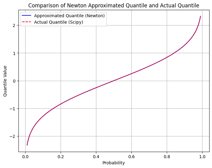

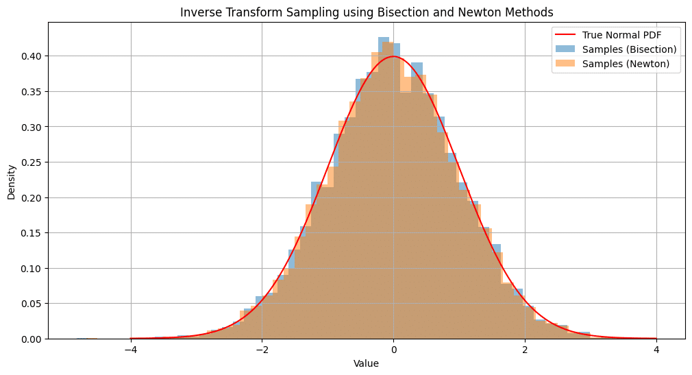
二分法、ニュートン法を用いた正規分布のCDFの逆関数の近似を用いた正規分布の逆関数法

import numpy as np
import matplotlib.pyplot as plt
from scipy.stats import norm

# 以前のセクションで定義したinverse_cdf（ビセクション法）とinverse_cdf_newton（ニュートン法）

# サンプル数
N = 10000

# 一様分布からのサンプル
uniform_samples = np.random.uniform(0, 1, N)

# ビセクション法を使ったサンプリング
samples_bisection = [inverse_cdf(p) for p in uniform_samples]

# ニュートン法を使ったサンプリング
samples_newton = [inverse_cdf_newton(p) for p in uniform_samples]

# プロット
plt.figure(figsize=(12, 6))

# 真の正規分布のPDF
x = np.linspace(-4, 4, 1000)
plt.plot(x, norm.pdf(x), 'r-', label='True Normal PDF')

# ビセクション法のヒストグラム
plt.hist(samples_bisection, bins=50, density=True, alpha=0.5, label='Samples (Bisection)')

# ニュートン法のヒストグラム
plt.hist(samples_newton, bins=50, density=True, alpha=0.5, label='Samples (Newton)')

plt.xlabel("Value")
plt.ylabel("Density")
plt.title("Inverse Transform Sampling using Bisection and Newton Methods")
plt.legend()
plt.grid(True)
plt.show()

この記事が気に入ったらサポートをしてみませんか？