
パンフレットスペックからモデルを作ってみよう! 「油圧ポンプ」

今回、パンフレットスペックからモデル化してみようと思ったきっかけは、友人の安藤博士から「実際にある油圧機器をモデルにしてみない?」という提案があったからです。確かに、パンフレットの情報からどこまでモデル化できるのかは興味があるなと思いチャレンジしてみることにしました。
今回のモデル化の立ち位置
モデル化をするときに一番大事なのはモデル化の立ち位置(目的)です。
この立ち位置があやふやですと、どんな粒度や精度のモデルを作ったらよいか定まりませんので、無駄に細かく作ろうとしたりするかもしれません。
なので、まずはモデル化の立ち位置を明確にしていきましょう。
今回は油圧機器を組み合わせた油圧システム全体の挙動を見たいという立ち位置で作成していきます。
なお、立ち位置が変わると作るモデルが変わってきます。油圧ポンプ自体の設計のための油圧ポンプモデルとなると、油を吸い上げて圧縮して送り出す機能や、吐き出し容量をコントロールする斜板角をコントロールするピストンの機能などポンプ1つを取っても多くの機能を設計していかなければなりません。一方で、ポンプを使ってシステムを設計する立ち位置でポンプをモデル化するとなると必要な機能は送り出される作動油量だけという場合もあります。モデル化する人が何を見たい(設計したい)かによって作るモデルが変わってくるので、まずはご自身が見たいものをよく考えてみるのがよいでしょう。
今回モデル化にチャレンジする油圧ポンプ
WEBページで情報が入手できた不二越さん(株式会社不二越)の可変容量形ピストンポンプ(PZSシリーズ)を入手できたパンフレットスペックから可能な範囲でモデル化をしてみたいと思います。
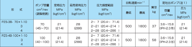
PZSシリーズにはいくつもの種類がありますので今回は一例としてPZS-4B-100R4S4-10をモデル化したいと思います。図1の2行目がPZS-4B-100R4S4-10のメインスペックです。「*1」の部分は仕様によっていくつかのパターンが用意されていますが、今回は「R4S4」としました。
「R4S4」はソレノイドカットオフ制御方式で、ソレノイド入力によってカットオフを制御します。「R4」は圧力制御範囲が2~28[MPa]を選択したいることを意味し、「S4」はソレノイド入力が24[V]を意味します。
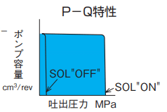
パンフレットの情報から、2~28[MPa]の圧力制御範囲は手動で最高圧を設定し、ソレノイドON(24[V])のときに最大圧でのP-Q特性となり、ソレノイドOFF(0[V])でカットオフ時のP-Q特性となります。
なお、私が読み取りが不十分かもしれませんので、その場合はお許しください。
今回のモデル化では、最大圧は28[MPa]としました。図2の絵からしかP-Q特性はわかりませんので、絵からの推測して、28[MPa]でポンプ容量はミニマム(図1より40[cc/rev])になるものとします。ポンプ容量の小さくなり始める圧力は27.5[MPa]とします。このあたりの正確なデータが必要な場合には油圧機器メーカー(今回でいうと不二越さん)に問い合わせて聞くと出してくれると思います。また、1DCAEによってシステム評価する際には、このあたりのスペックの個体差をばらつかせてシステム性能への影響を評価しておくとよいでしょう。
ソレノイドOFF(カットオフ)時のP-Q特性も同様に、ポンプ圧がミニマムになるポンプ圧力をポンプの圧力制御範囲の最小値である2[MPa]として、ポンプ容量が小さくなり始める圧力を最大側と同じく0.5[MPa]の差として1.5[MPa]からポンプ容量を小さくなるようにします。
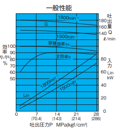
容積効率も図3の絵からしか判断できませんので、ざっくりと7[MPa]まで100%、28[MPa]で92%になるようにします。
機械効率は全効率を容積効率で割れば出ますが、低圧側は元のエネルギーが少ないためにかなり低くなっていますが、そもそものエネルギーが低いため、この領域でメインで使ってかつトルク管理をする必要はなければあまり気にする必要はないと思います。トルクが小さい領域なので、思い切って無視してざっくりと一律90%にします。
なお、図3のデータは作動油の動粘度が46[㎟/s]のときのデータです。通常使用領域と思えば普段は気にしないでよいですが、著しく変わってきてしまう場合には性能が変化しますので、その際は性能の変化を見込んだシミュレーションもしておくと間違いないでしょう。
あと、ソレノイドによる応答性の情報がパンフレットには記載がなかったので、100[ms]の一次遅れ応答としておきます。
今回のモデル化では、以上の条件でモデル化をしてみます。
今回のモデル化には使わないけど大事な情報
ポンプ吸入側圧力は-0.03[MPa]以上(吸入ポート流速は2[m/sec]以
内)。
これは吸入側の圧力が負圧になりすぎない条件です。ポンプの吐出し量に対応できる作動油を吸入側に確保できる構造にしなければならないということです。必要に応じて吸入側へ作動油を確保させる補助装置を設ける場合もあるかもしれません。
ドレン背圧が0.1MPa以下。
これはポンプのケース内に漏れ出した作動油を作動油タンクに戻すラインのことですが、規定の圧以下にしないと適正にタンクに戻せずに破損の原因になるかもしれませんし、ポンプの機械的な潤滑にも使っていたりするかもしれませんので、ゴミを適正に排出できないことで破損の原因になるかもしれません。メイン性能検討時は考えなくてもよいですが、最終的なモノづくり時には必ず規定を満たすように設計しましょう。
ポンプの吐出側にはチェックバルブを設ける(電動機OFF時の逆回転防止、ポンプの破損防止)。
これは記載のとおり逆回転防止です。ちょっとだけ気にしなけばならないことは、チェックバルブの圧損です。リリーフバルブをチェックバルブの出口側のラインに設置した場合、ポンプの吐き出し側はリリーフ圧にチェックバルブの圧損分だけ高くなる場合がありますから、ポンプの耐圧のことを少し考えておく必要があります。
作動油の管理
品質が良好な作動油を用いて、使用時の動粘度は20~200[㎟/s]の範囲で使用。一般には、R&Oタイプ、耐摩耗性タイプのISOVG32~68相当品を使用。
運転時の最適動粘度範囲は20~50[㎟/s]。使用温度範囲は5~60°C。起動時の油温が5°C以下の場合は、低圧低速回転で油温が5°Cになるまで暖気運転を行う。サクションストレーナは、ろ過粒度100μ(150メッシュ)程度のものを使用。作動油の汚染度はNAS10級以下を保つよう管理。使用周囲温度0~60°C。
このポンプは低温側(マイナス温度)の制約から、氷点下になる寒冷地では温度対策をしないと使用できないことがわかります。
また、作動油性能がしっかり規定されていますので、劣悪な作動油を使われてしまう地域での使用は難しいかもしれませんね。
MapleSimでモデル化
最初に言ったとおり、今回は油圧機器を組み合わせた油圧システム全体の挙動を見たいという立ち位置で作成していきます。要するに今回の場合、ポンプから吐き出される流量変化がわかればよいというスタンスでモデル化を行います。なので、ポンプに含まれる細かい油圧機器のモデル化は行いません。なお、パンフレット内にもどのようなポンプ斜板制御をしているのかがざっとわかるようなポンプ内の油圧回路が記載されていますので、ポンプ内での動作はある程度想像できますので、興味がある方はパンフレットを参照してみてください。
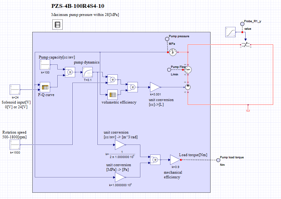
さて、モデル化の本題ですが、まずは図4に最終系のモデルを見せちゃいます。そして後段で内部を説明していきます。
図4に示しているモデルには、作成したモデルを動かすために必要な入力(ソレノイド入力とポンプの入力軸回転数)と、ポンプ圧によるポンプの動きの違いを見るために、ポンプの吐き出し側に絞り弁をつけています。ポンプ部分は背景色を変えている部分になります。なお、みなさんが使う場合には背景色を変えてある部分をサブシステム化しておくと油圧システム全体の見通しはよくなるかもしれませんね。
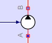
MapleSimにあるポンプ流量を変えられる油圧ポンプブロックを図5に示します。ブロックへの横からの入力で流量自体を指定しなければならないので、現在の状況による流量を計算する部分を別途作る必要があります。
ここで、今回作成するポンプの流量変化に影響を与える機能をまとめておきます。
(1)P-Q特性(ポンプ圧が高まるとポンプ吐き出し流量が減少する特性)
(2)ソレノイド入力によるP-Q特性の切り替え
(3)ポンプ斜板機構の応答性
(4)容積効率(吐き出される流量の効率)
図6はP-Q特性、ソレノイド入力による切替、斜板機構の応答性の計算部分を表しています。「Pump capacity」はポンプの最大容量として100[cc/rev]としています。「P-Q curve」はポンプ圧とソレノイド入力によってP-Q特性(ポンプ容量の低減率)を算出します。算出したP-Q特性の値をポンプの最大容量に掛け算することでポンプ容量の定常値を算出します。その値を一次遅れ応答(「pump dynamics」)に入力して応答性を表現しています。ポンプの斜板機構の応答性についてはパンフレットに記載がなかったので、本モデルでは100[ms]の一次遅れ応答としました。
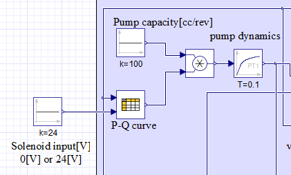
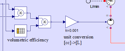
図7を見ると、先ほど算出したポンプ容量(一次遅れ応答後)とポンプの入力軸回転数との積(左側の掛け算ブロック)によりポンプ流量を算出しています。さらに現在のポンプ圧から求めた容積効率(「volumetric efficiency」)と算出したポンプ流量との積(右側の掛け算ブロック)により容積効率を加味したポンプ流量を算出しています。最後のゲインブロックは流量の単位を「cc」から「L」に換算してポンプブロックに入力しています。
今回はポンプから吐き出される流量だけでなく、ポンプを動かすエンジンや電動機への負荷トルクもモデル化します(図8)。ポンプの負荷トルクを計算しておくことで、ポンプ圧が上昇した時のエンジン回転ダウンなどを検討することができます。トルク応答性の高い電動機でポンプを回している場合には、ポンプの入力軸回転数はあまり変動しない場合もあるので、その場合には一定回転をポンプに入力しておいてよいでしょう。
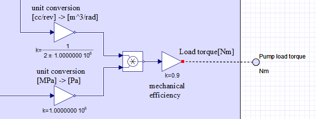
図8の上側のラインはポンプ容量でゲインは単位換算をしています。図8の下側はポンプ圧でゲインは同じく単位換算をしています。ポンプの負荷トルクはポンプ圧とポンプ容量の積で計算できます。掛け算ブロックの後段のゲインは機械効率(一律90%)です。
なお、正しくはポンプの吸い込み側の圧に対するポンプの出力側の圧とポンプ容量の積とすべきですが、ポンプの吸い込み側の圧を0[MPa]と仮定しているので、本モデルではポンプ圧とポンプ容量との積でポンプの負荷トルクを算出しています。
作動油の特性を図9に示しておきます。
体積弾性率Kを14000[bar]、動粘度vをポンプのパンフレット性能の値(0.000046[㎟/s])にしておきます。なお、密度ρはデフォルトのままです。
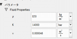
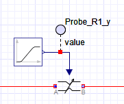
図10はポンプ圧を上昇させるための絞り弁です。時間の経過とともに開口面積を絞っていくので、ポンプ圧が上昇していきます。
シミュレーションをしてみよう
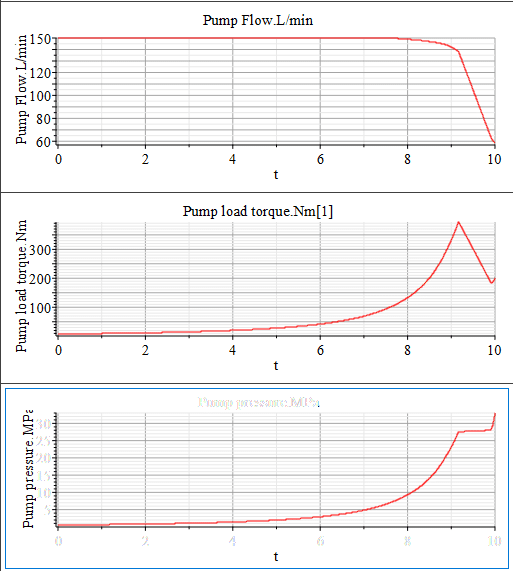
シミュレーション結果を図11に示します。
絞り弁を徐々に絞っていくことでポンプ圧を上げていくと27.5[MPa]を超えるとポンプ容量が絞られているのがわかります。ポンプ容量が最小になってもさらに絞られると圧が抑えられず急上昇していいます。
また、27.5[MPa]前にも7[MPa]を超えるとポンプ容量が低下しているのは容積効率が低下しているからなのです。そのため、ポンプの負荷トルクは、ポンプ容量が小さくなり始めると低下していっているのがわかります。最後の方でポンプトルクが上昇しているのは、ポンプ容量がミニマム底打ちになって、ポンプ圧が上がっているために上昇しています。
【English】
The reason I decided to try modeling from pamphlet specs this time was a suggestion from my friend Dr. Ando, "Why don't we model actual hydraulic equipment?" I decided to give it a try because I was curious to see how far I could go in modeling from the information in the pamphlet.
Standing point of this modeling
When modeling, the most important thing to consider is the standing point (objective) of the modeling. If this position is unclear, it is difficult to determine what granularity and precision of the model should be created, and you may try to create a detailed model in vain. Therefore, let's first clarify the standing point of modeling. This time, we will create a model from the standpoint that we want to see the behavior of the entire hydraulic system combining hydraulic equipment.
The model to be created changes as the position changes. A hydraulic pump model for designing a hydraulic pump itself requires the design of many functions even for a single pump, such as the function of sucking up, compressing, and sending out oil, and the function of the piston that controls the swash plate angle to control the discharging capacity. On the other hand, when a pump is modeled from the standpoint of designing a system using a pump, the only function required may be the amount of hydraulic oil to be pumped. The model to be created will depend on what the modeler wants to see (design), so it is a good idea to first carefully consider what you want to see.
Hydraulic pump to be modeled this time
I would like to model the variable displacement type piston pump (PZS series) of NACHI Ltd. for which information was available on the web page to the extent possible from the available pamphlet specifications.
There are a number of different types in the PZS series, so I would like to model PZS-4B-100R4S4-10 as an example this time. The second line in Figure 1 shows the main specifications of the PZS-4B-100R4S4-10. The "*1" part has several patterns depending on the specifications, but in this case, "R4S4" is used.
R4S4" is a solenoid cutoff control type, where the cutoff is controlled by the solenoid input. R4" means that the pressure control range of 2 to 28 [MPa] is selected, and "S4" means that the solenoid input is 24 [V].
Based on the information in the pamphlet, the pressure control range of 2 to 28[MPa] is the P-Q characteristic at maximum pressure when the maximum pressure is manually set and the solenoid is ON (24[V]), and the P-Q characteristic at cutoff when the solenoid is OFF (0[V]).
Please note that my reading of the pamphlet may be inadequate and incorrect, in which case please forgive me.
In this modeling, the maximum pressure was set at 28[MPa]. Since the P-Q characteristic is known only from the picture in Figure 2, it is assumed that the pump capacity is at minimum (40 [cc/rev] from Figure 1) at 28 [MPa] by inference from the figure. The pressure at which the pump capacity starts to decrease is assumed to be 27.5[MPa]. If you need accurate data in this area, contact the hydraulic equipment manufacturer (in this case, NACHI Ltd.) and ask them. Also, when evaluating a system by 1DCAE, it is advisable to vary the individual differences in specifications in this area to evaluate the impact on system performance.
Similarly, the P-Q characteristic when the solenoid is turned off (cutoff) is set to 2[MPa], the minimum value of the pump pressure control range, where the pump pressure becomes minimal, and the pressure at which the pump capacity begins to decrease is set from 1.5[MPa].
The volumetric efficiency can only be determined from Figure 3, so it is roughly modeled as 100% up to 7[MPa] and 92% at 28[MPa].
The mechanical efficiency can be obtained by dividing the volumetric efficiency from the total efficiency. The low pressure side is quite low because of the low base energy. Since the base energy is low, we do not need to worry too much about this area unless we need to use this area as a major application or to manage torque. In this case, since the torque is small in this area, we will boldly ignore it and set it roughly at 90% uniformly.
Note that the data in Figure 3 is for a kinematic viscosity of 46[㎟/s] of hydraulic oil. If it is considered as a normal use area, it is not usually necessary to worry about it, but if it changes significantly, the performance will change, so it is surely better to simulate the change in performance in such cases.
Also, there was no information in the pamphlet about the responsiveness due to the solenoid, so I will assume a primary delay response of 100[ms]. In this modeling, I will try to model the above conditions.
Information that will not be used for this modeling but is important
The pump suction side pressure is -0.03 [MPa] or higher (suction port flow velocity is within 2 [m/sec]). This is a condition where the suction side pressure is not too negative. It means that the structure must be capable of sending enough hydraulic oil to the suction side to be sufficient for the discharge volume of the pump. If necessary, an auxiliary device may be installed to satisfy the hydraulic oil to the suction side.
Drain back pressure is less than 0.1 MPa. This refers to the line that returns the hydraulic oil leaked into the pump case to the hydraulic oil tank, but if the pressure is not below the specified pressure, it may not be returned to the tank properly, which may cause damage. This may cause damage if the pump is not properly drained of debris. It is not necessary to consider this when considering the main performance, but be sure to design the product to meet the regulations when making the final manufacturing.
Provide a check valve on the outlet side of the pump (to prevent reverse rotation when the electric motor is turned off and to prevent damage to the pump). This is to prevent reverse rotation as described. A slight concern is the pressure drop across the check valve. If a relief valve is installed in the line on the outlet side of the check valve, the relief pressure on the outlet side of the pump may be higher than the relief pressure by the pressure loss of the check valve.
Hydraulic fluid management
Use high quality hydraulic oil, with kinematic viscosity in the range of 20 to 200 [㎟/s] when in use. Generally, R&O type, wear-resistant type ISOVG 32-68 or equivalent is used. The optimum kinematic viscosity range for operation is 20 to 50 [㎟/s]. Operating temperature range is 5 to 60°C. If the oil temperature at startup is below 5°C, warm-up operation should be performed at low pressure and low speed until the oil temperature reaches 5°C. Suction strainers should be used with a filtration particle size of about 100μ (150 mesh). The degree of contamination of the hydraulic oil should be kept below NAS 10. Ambient operating temperature 0 to 60°C.
The restrictions on the low temperature side (minus temperature) of this pump indicate that it cannot be used in cold regions where the temperature drops below freezing without temperature countermeasures. Also, since the hydraulic oil performance is well specified, it may be difficult to use in regions where inferior hydraulic oil would be used.
Modeling with MapleSim
As I said at the beginning, this time we will create the model from the standpoint that we want to see the behavior of the entire hydraulic system combining hydraulic devices. In short, in this case, we will model the system from the standpoint that it is sufficient to understand the changes in the flow rate discharged from the pump. Therefore, we will not model the detailed hydraulic components included in the pump. The pamphlet also describes the hydraulic circuit inside the pump to give a rough sketch of how the pump swash plate is controlled, so you can imagine the operation of the pump to some extent.
Now for the main part of the modeling, I'm going to show the complete model in Figure 4 first. Then I will explain the internals in a later section. The model shown in Figure 4 has the inputs required to run the created model (solenoid input and pump input shaft speed) and an orifice on the discharge side of the pump to see the difference in pump movement due to pump pressure. The pump part is the part whose background color is changed. In case you use this model, it may be better to subsystem the part with the different background color to get a better view of the entire hydraulic system.
A hydraulic pump block in MapleSim that can change the pump flow rate is shown in Figure 5. Since the flow rate itself must be specified in the side input to the block, a separate section must be created to calculate the flow rate due to the current conditions.
Here is a summary of the functions that affect the flow rate variation of the pump to be created in this case.
(1) P-Q characteristic (the characteristic that the pump discharge flow rate decreases as the pump pressure increases)
(2) P-Q characteristic switching by solenoid input
(3) Responsiveness of the pump swash plate mechanism
(4) Volumetric efficiency (efficiency of discharged flow rate)
Figure 6 shows the P-Q characteristics, switching by solenoid input, and the responsiveness calculation part of the swash plate mechanism. The "Pump capacity" is set to 100 [cc/rev] as the maximum pump capacity. The "P-Q curve" calculates the P-Q characteristic (reduction rate of pump capacity) based on the pump pressure and solenoid input. The calculated P-Q characteristic value is multiplied by the maximum pump capacity to calculate the steady-state value of the pump capacity. That value is input to the primary delay response ("pump dynamics") to express the responsiveness. Since the response of the swash plate mechanism of the pump was not described in the pamphlet, a first-order delay response of 100[ms] was used in this model.
Figure 7 shows that the product of the pump capacity (after primary delay response) calculated earlier and the pump input shaft speed (left-hand multiplication block) is used to calculate the pump flow rate. Furthermore, the product of the volumetric efficiency ("volumetric efficiency") calculated from the current pump pressure and the calculated pump flow rate (the multiplication block on the right) is used to calculate the pump flow rate with the volumetric efficiency added. The last gain block converts the flow rate unit from "cc" to "L" and inputs it to the pump block.
This time, not only the flow rate discharged from the pump, but also the load torque on the engine or electric motor that runs the pump is modeled (Figure 8). By calculating the load torque on the pump, it is possible to consider such factors as engine rotation down when pump pressure increases. If the pump is run by an electric motor with high torque response, the input shaft speed of the pump may not fluctuate much, in which case a constant rotation may be input to the pump.
The upper line in Figure 8 is the pump capacity and the gain is converted to units. The lower line in Figure 8 is the pump pressure, and the gain is also converted to units. The load torque of the pump can be calculated as the product of pump pressure and pump capacity. The gain in the second part of the multiplication block is the mechanical efficiency (uniformly 90%). Note that the correct value should be the product of the pressure on the outlet side of the pump and the pump capacity relative to the pressure on the suction side of the pump, but since the pressure on the suction side of the pump is assumed to be 0 [MPa], the load torque of the pump is calculated as the product of the pump pressure and the pump capacity in this model.
The characteristics of the hydraulic oil are shown in Figure 9. The volume modulus K is set to 14000 [bar] and the kinematic viscosity v to the pamphlet performance value of the pump (0.000046 [㎟/s]). Note that the density ρ is left at the default value.
Figure 10 shows an orifice for increasing pump pressure. As the opening area is narrowed over time, the pump pressure increases.
Let's run a simulation
Simulation results are shown in Figure 11. When the pump pressure is increased by gradually closing the orifice opening area, it can be seen that the pump capacity is reduced when it exceeds 27.5 [MPa]. Even after the pump capacity reaches its minimum, if the orifice opening area is further reduced, the pressure increase cannot be controlled and rises sharply. Also, the pump capacity decreases before 27.5[MPa] and after 7[MPa] because the volumetric efficiency is decreasing. Therefore, we see that the load torque of the pump is decreasing as the pump capacity starts to decrease. The pump torque is increasing at the end because the pump capacity is bottoming out minimally and the pump pressure is increasing.
【Sample】
Created by MapleSim 2023
この記事が気に入ったらサポートをしてみませんか?