【Python】投資部門別売買動向の可視化

海外投資家、個人投資家、機関投資家が買い越している、売り越しているというのをニュースやネット記事で見聞きします。
ここでは、JPX(日本取引所グループ)の統計情報(株式関連)(リンク参照)の投資部門別売買状況のページ(リンク参照)から金額ベースの売買状況データをダウンロードして、Plotlyを使って可視化していきます。この情報は、毎週第4営業日(通常は木曜日、祝日等非営業日がある場合はその分後ろ倒し) 午後3時に資料が更新して掲載されています。
なお、最低限のポイントのみの説明にするため、Pythonライブラリ、モジュール等のインストール方法については割愛させて頂きます。お使いのPC環境等に合わせてインストールしてもらえればと思います。
1.株式売買状況データの取得方法
週間データが、JPX(日本取引所グループ)の投資部門別売買状況ページ(下記リンク参照)にあります。
投資部門別売買状況 | 日本取引所グループ (jpx.co.jp)
リンクを開くとエクセルとpdfでダウンロードできるページが現れますので、ここからデータを落としていきます。金額と書かれている方が売買代金、株数と書かれている方が出来高ということになります。今回は、金額と書かれているエクセルファイルをダウンロードします。
なお、ここでは、2023年の10月の1週目から2023年の12月の3週目までの各週ごとのデータをダウンロードしてdataフォルダに格納しておきます。
|-data
|-stock_val_1_231001.xls (2023年10月の1週目のデータ)
|-stock_val_1_231002.xls (2023年10月の2週目のデータ)
|-stock_val_1_231003.xls (2023年10月の3週目のデータ)
|-stock_val_1_231004.xls (2023年10月の4週目のデータ)
|-stock_val_1_231101.xls (2023年11月の1週目のデータ)
|-stock_val_1_231102.xls (2023年11月の2週目のデータ)
|-stock_val_1_231103.xls (2023年11月の3週目のデータ)
|-stock_val_1_231104.xls (2023年11月の4週目のデータ)
|-stock_val_1_231105.xls (2023年11月の5週目のデータ)
|-stock_val_1_231201.xls (2023年12月の1週目のデータ)
|-stock_val_1_231202.xls (2023年12月の2週目のデータ)
|-stock_val_1_231203.xls (2023年12月の3週目のデータ)
2.株式売買状況データの詳細
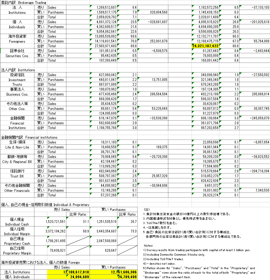
データの中身を開いてみると以下のようなデータが得られていると思います。示しているデータは2023年12月3週目(12/18〜12/22)のデータです。金額の単位は千円です。H列からK列が2023年12月3週目(12/18〜12/22)のデータとなっています。D列からG列は前週のデータなので、H列からK列のデータを確認してデータ取得していきます。
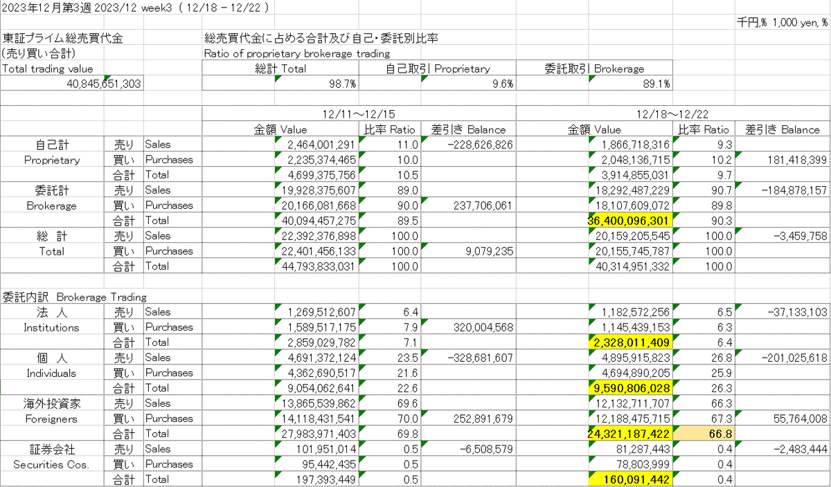
① 東証プライム総売買代金(Total trading value)
12/18〜12/22の合計売買代金(千円)です。
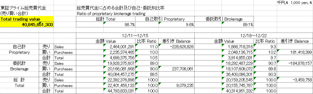
② 自己取引(Proprietary)
「証券会社や銀行などが、自分の勘定を使って株式や債券、為替などに投資すること」のようです。
【参考】https://www.weblio.jp/content/%E8%87%AA%E5%B7%B1%E5%A3%B2%E8%B2%B7
③ 委託取引(Brokerage)
「商品の販売や買付を、一定の手数料を払って第三者の代行機関に委託すること」。我々のような個人投資家が証券会社を経由して取引するのはこちらになるようです。
【参考】https://www.weblio.jp/content/%E5%A7%94%E8%A8%97%E5%A3%B2%E8%B2%B7
④ 差引き(Balance)
(買い金額)ー(売り金額)を示しています。このデータの総計のところを見ると、34億円ほど売り越していることがわかります。
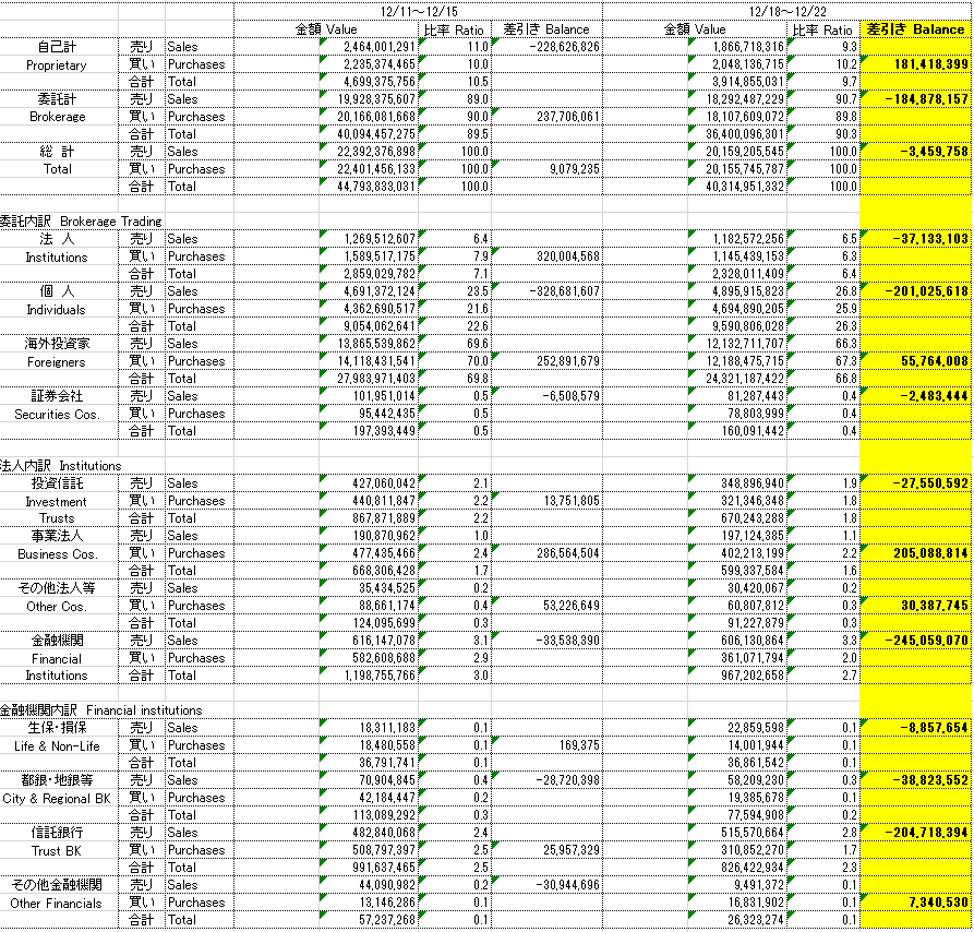
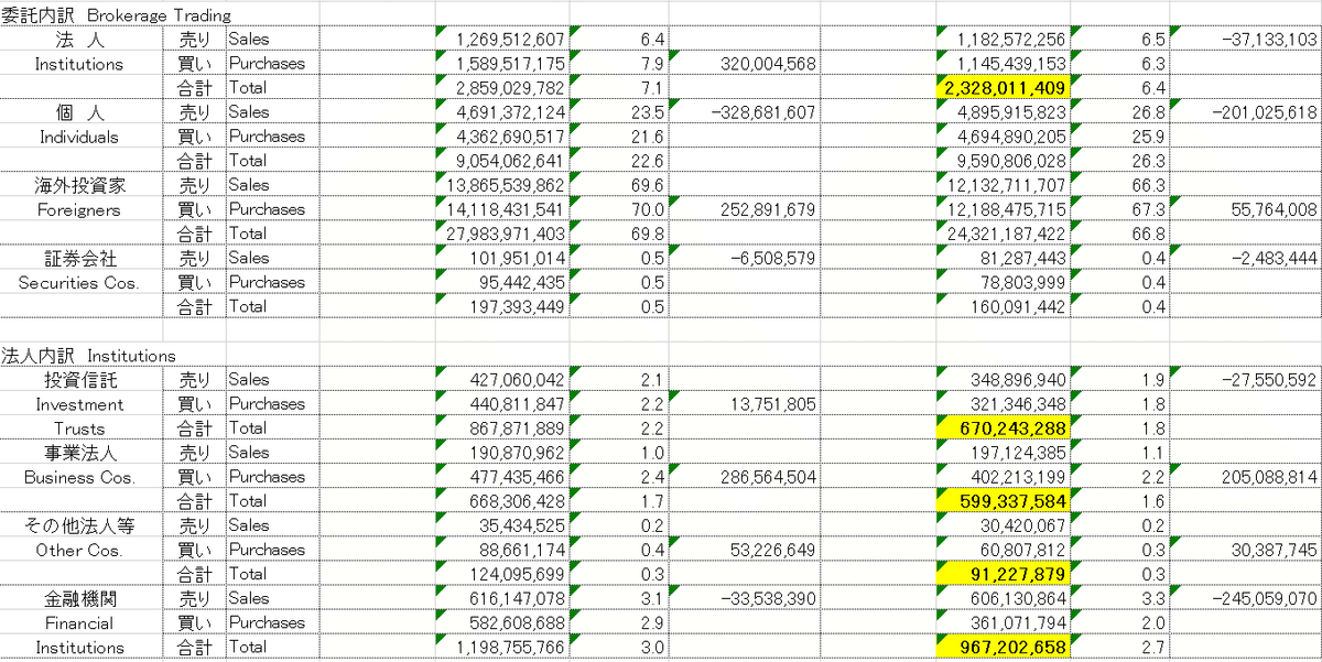
⑤ 委託内訳(Brokerage Trading)
委託取引の内訳が記載されており、法人(Institutions)、個人(Individuals)、海外投資家(Foreigners)、証券会社(Securities Cos.)に分かれております。委託取引の内訳を示しているので、セルI26、I29、I32、I35を合計するとI18になります。この内訳の中で、海外投資家のTotalの部分の比率を見てみると66.8%となっており、委託取引のうちの7割弱が海外投資家の取引ということになります。
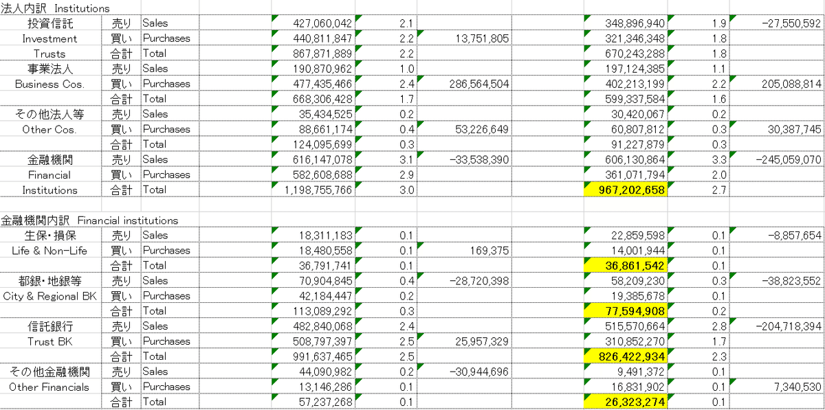
⑥ 法人内訳(Institutions)
委託内訳(Brokerage Trading)の法人の部分に関して、さらに細かい内訳が示されており、投資信託(Investment)、事業法人(Business Cos.)、その他法人等(Other Cos.)、金融機関(Financial Institutions)からなっています。委託取引の中の法人の内訳なので、セルI40、I43、I46、I49を合計するとI26になります。
⑦ 金融機関内訳(Finantial Institutions)
法人内訳(Institutions)の中の金融機関(Financial Institutions)の部分に関して、さらに細かく内訳が示されています。生保・損保(Life & Non-Life)、都銀・地銀(City & Regional BK)、信託銀行(Trust BK)、その他金融機関(Other Financials)からなっています。⑤⑥同様に、I54、I57、I60、I63を合計するとI49になります。
⑧ 個人と自己売買、それぞれの現金取引か信用取引の売買金額を示しております。C68、C69、E68、E69を合計するとI29になります。またC70、C71、E70、E71を合計するとI15になります。

⑨ 海外投資家売買における法人、個人の数値(Foreign)
海外投資家の法人(Institutions)と個人( Individuals)の売買金額が示されています。D75、D76、F75、76を合計するとI32になります。
海外投資家の取引が重要であることはエクセルから確認できました。これを時系列データとして可視化することで、より詳細な売買動向がわかってきます。
3.売買動向データを取得してデータフレームにする
dataフォルダから、各年月週のエクセルデータを読み込んでデータフレームを作成していきます。
|-data
|-stock_val_1_231001.xls
|-stock_val_1_231002.xls
|-stock_val_1_231003.xls
|-stock_val_1_231004.xls
|-stock_val_1_231101.xls
|-stock_val_1_231102.xls
|-stock_val_1_231103.xls
|-stock_val_1_231104.xls
|-stock_val_1_231105.xls
|-stock_val_1_231201.xls
|-stock_val_1_231202.xls
|-stock_val_1_231203.xls
各種ライブラリをインポートします。
xlrd:Excel (xls) のデータを Python で読むためのライブラリ
glob:ファイルをパスを取得するライブラリ
plotly.graph_objects:グラフを可視化するPlotlyライブラリ
import pandas as pd
import xlrd
import glob
import plotly.graph_objects as go次にデータのパスを取得して、filesにリストとして格納します。今後、for文でfilesリストの中身のパスをまわして、データにアクセスしていきます。
#dataフォルダ内のエクセルファイルのpathをfilesに格納
files = sorted(glob.glob('data/*'))
print(files)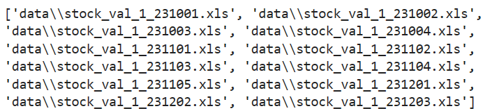
エクセルファイルのデータを格納していく辞書 dict_inventor を作成して初期化します。
dict_inventor = {
    'ProprietarySales':0,  # 自己計_売
    'ProprietaryPurchases':0,  #自己計_買
    'ProprietaryTotal':0,  # 自己計_合計

    'BrokerageSales':0,  # 委託計_売
    'BrokeragePurchases':0,  # 委託計_買
    'BrokerageTotal':0,  # 委託計_合計

    'TotalSales':0,  # 総計_売
    'TotalPurchases':0,  # 総計_買
    'TotalTotal':0,  # 総計_合計

    'IndividualsSales':0,  # 個人_売
    'IndividualsPurchases':0,  # 個人_買
    'IndividualsTotal':0,  # 個人_合計

    'ForeignersSales':0,  # 海外投資家_売
    'ForeignersPurchases':0,  # 海外投資家_買
    'ForeignersTotal':0,  # 海外投資家_合計

    'SecuritiesCosSales':0,  # 証券会社_売
    'SecuritiesCosPurchases':0,  # 証券会社_買
    'SecuritiesCosTotal':0,  # 証券会社_合計

    'InvestmentTrustsSales':0,  # 投資信託_売
    'InvestmentTrustsPurchases':0,  # 投資信託_買
    'InvestmentTrustsTotal':0,  # 投資信託_合計

    'BusinessCosSales':0,  # 事業法人_売
    'BusinessCosPurchases':0,  # 事業法人_買
    'BusinessCosTotal':0,  # 事業法人_合計

    'OtherCosSales':0,  # その他法人_売
    'OtherCosPurchases':0,  # その他法人_買
    'OtherCosTotal':0,  # その他法人_合計

    'InsuranceCosSales':0,  # 生保・損保_売
    'InsuranceCosPurchases':0,  # 生保・損保_買
    'InsuranceCosTotal':0,  # 生保・損保_合計

    'CityBKsRegionalBKsEtcSales':0,  # 都銀・地銀等_売
    'CityBKsRegionalBKsEtcPurchases':0,  # 都銀・地銀等_買
    'CityBKsRegionalBKsEtcTotal':0,  # 都銀・地銀等_合計

    'TrustBanksSales':0,  # 信託銀行_売
    'TrustBanksPurchases':0,  # 信託銀行_買
    'TrustBanksTotal':0,  # 信託銀行_合計

    'OtherFinancialInstitutionsSales':0,  # その他金融機関_売
    'OtherFinancialInstitutionsPurchases':0,  # その他金融機関_買
    'OtherFinancialInstitutionsTotal':0,  # その他金融機関_合計
}filesリストの中身のパスをfor文でまわして、エクセルファイルデータのセルの値を取得して、上記で定義した辞書 dict_inventor に格納していきます。
また、年月週は、forループの中で、dataフォルダにある読み込むファイル名から取得して変数dateに格納します。例えば、stock_val_1_231001.xls の場合、後ろから10文字目から後ろから4文字より前までの文字列を取り出して格納します。date_list.append(date) することで、date_list に格納されます。
辞書 dict_inventor をデータフレームに変換して df を作成します。
df = pd.DataFrame()  # 空のデータフレームを作成
date_list = []  # 年月週を格納するリスト

for i in range(len(files)):
    file = files[i]
    wb = xlrd.open_workbook(file)
    sheet_names = wb.sheet_names()
    sheet = wb.sheet_by_name(sheet_names[0])

    # 後ろから10文字目から後ろから4文字より前までの文字列を取り出して、変数dateに格納
    date = file[-10:-4]
    date_list.append(date)

    print(file)
    print(date)


    # エクセルシートから値を取得して辞書に格納

    # 自己計(Proprietary)
    dict_inventor['ProprietarySales'] = sheet.cell(12,8).value
    dict_inventor['ProprietaryPurchases'] = sheet.cell(13,8).value
    dict_inventor['ProprietaryTotal'] = sheet.cell(14,8).value

    # 委託計(Brokerage)
    dict_inventor['BrokerageSales'] = sheet.cell(15,8).value
    dict_inventor['BrokeragePurchases'] = sheet.cell(16,8).value
    dict_inventor['BrokerageTotal'] = sheet.cell(17,8).value

    # 総計(Total)
    dict_inventor['TotalSales'] = sheet.cell(18,8).value
    dict_inventor['TotalPurchases'] = sheet.cell(19,8).value
    dict_inventor['TotalTotal'] = sheet.cell(20,8).value

    # 委託内訳
    # 個人
    dict_inventor['IndividualsSales'] = sheet.cell(26,8).value
    dict_inventor['IndividualsPurchases'] = sheet.cell(27,8).value
    dict_inventor['IndividualsTotal'] = sheet.cell(28,8).value

    # 海外投資家
    dict_inventor['ForeignersSales'] = sheet.cell(29,8).value
    dict_inventor['ForeignersPurchases'] = sheet.cell(30,8).value
    dict_inventor['ForeignersTotal'] = sheet.cell(31,8).value

    # 証券会社
    dict_inventor['SecuritiesCosSales'] = sheet.cell(32,8).value
    dict_inventor['SecuritiesCosPurchases'] = sheet.cell(33,8).value
    dict_inventor['SecuritiesCosTotal'] = sheet.cell(34,8).value

    #法人内訳
    # 投資信託
    dict_inventor['InvestmentTrustsSales'] = sheet.cell(37,8).value
    dict_inventor['InvestmentTrustsPurchases'] = sheet.cell(38,8).value
    dict_inventor['InvestmentTrustsTotal'] = sheet.cell(39,8).value

    # 事業法人
    dict_inventor['BusinessCosSales'] = sheet.cell(40,8).value
    dict_inventor['BusinessCosPurchases'] = sheet.cell(41,8).value
    dict_inventor['BusinessCosTotal'] = sheet.cell(42,8).value

    # その他法人
    dict_inventor['OtherCosSales'] = sheet.cell(43,8).value
    dict_inventor['OtherCosPurchases'] = sheet.cell(44,8).value
    dict_inventor['OtherCosTotal'] = sheet.cell(45,8).value

    #金融機関売買の内訳
    # 生保・損保
    dict_inventor['InsuranceCosSales'] = sheet.cell(51,8).value
    dict_inventor['InsuranceCosPurchases'] = sheet.cell(52,8).value
    dict_inventor['InsuranceCosTotal'] = sheet.cell(53,8).value

    # 都銀・地銀等
    dict_inventor['CityBKsRegionalBKsEtcSales'] = sheet.cell(54,8).value
    dict_inventor['CityBKsRegionalBKsEtcPurchases'] = sheet.cell(55,8).value
    dict_inventor['CityBKsRegionalBKsEtcTotal'] = sheet.cell(56,8).value

    # 信託銀行
    dict_inventor['TrustBanksSales'] = sheet.cell(57,8).value
    dict_inventor['TrustBanksPurchases'] = sheet.cell(58,8).value
    dict_inventor['TrustBanksTotal'] = sheet.cell(59,8).value

    # その他金融機関
    dict_inventor['OtherFinancialInstitutionsSales'] = sheet.cell(60,8).value
    dict_inventor['OtherFinancialInstitutionsPurchases'] = sheet.cell(61,8).value
    dict_inventor['OtherFinancialInstitutionsTotal'] = sheet.cell(62,8).value

    # 法人の集計(投資信託 + 事業法人 + その他法人 + 金融機関(生保・損保 + 都銀・地銀等 + 信託銀行 + その他金融機関))
    dict_inventor['InstitutionsSales'] = dict_inventor['InvestmentTrustsSales'] + dict_inventor['BusinessCosSales'] + dict_inventor['OtherCosSales'] + dict_inventor['InsuranceCosSales'] + dict_inventor['CityBKsRegionalBKsEtcSales'] + dict_inventor['TrustBanksSales'] + dict_inventor['OtherFinancialInstitutionsSales']
    dict_inventor['InstitutionsPurchases'] = dict_inventor['InvestmentTrustsPurchases'] + dict_inventor['BusinessCosPurchases'] + dict_inventor['OtherCosPurchases'] + dict_inventor['InsuranceCosPurchases'] + dict_inventor['CityBKsRegionalBKsEtcPurchases'] + dict_inventor['TrustBanksPurchases'] + dict_inventor['OtherFinancialInstitutionsPurchases']
    dict_inventor['InstitutionsTotal'] = dict_inventor['InvestmentTrustsTotal'] + dict_inventor['BusinessCosTotal'] + dict_inventor['OtherCosTotal'] + dict_inventor['InsuranceCosTotal'] + dict_inventor['CityBKsRegionalBKsEtcTotal'] + dict_inventor['TrustBanksTotal'] + dict_inventor['OtherFinancialInstitutionsTotal']


    sr = pd.Series(dict_inventor)  # 辞書をシリーズに変換
    df_tmp=pd.DataFrame(pd.Series(sr)).T  # 行と列を入れ替え
    df = pd.concat([df, df_tmp], ignore_index=True)  # ループでデータを結合

display(df)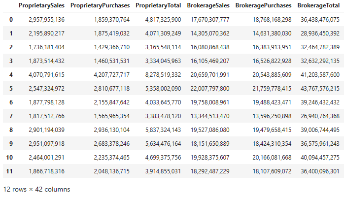
結合されたデータフレーム df を確認すると、エクセルデータから取得した値はカンマがついた文字列になっているので、あとでグラフにすることを考慮してカンマを除いたうえでfloat型の数値に変換します。さらにdate_list に格納された年月週も df に追加しておきます。
for key in dict_inventor.keys():
    df[key] = df[key].str.replace(',','').astype(float)

print(date_list)
df['date'] = date_list
4.売買動向データの可視化
次に、plotlyを使ってグラフに表示していきます。plotlyについては、以前に描画方法と見た目に関わる設定について投稿しているので参考にしてもらえればと思います。
4-1. 各投資家のトータルの売買代金の可視化
# グラフィック系ライブラリ
import plotly.graph_objects as go  # グラフ表示関連ライブラリ
import plotly.io as pio  # 入出力関連ライブラリ
pio.renderers.default = 'iframe'

# グラフの実体trace オブジェクトを生成
bar_trace_1 = go.Bar(x = df['date'], y = df['TotalSales'], name = 'TotalSales',yaxis='y1')
bar_trace_2 = go.Bar(x = df['date'], y = df['TotalPurchases'], name = 'TotalPurchases',yaxis='y1')
scatter_trace_1 = go.Scatter(x = df['date'], y = df['TotalSales'] - df['TotalPurchases'] , name = 'balance',  yaxis='y2')

# レイアウトオブジェクトを生成
graph_layout = go.Layout(

    # 幅と高さの設定
    width=1000, height=600,

    # タイトルの設定
    title=dict(
        text='各投資家トータルの売買動向', # タイトル
        font=dict(family='Times New Roman', size=20, color='grey'), # フォントの指定
        xref='paper', # container or paper
        x=0.5,
        y=0.87,
        xanchor='center',
    ),

    # 軸の設定
    xaxis = dict(showgrid=False),
    yaxis = dict(title = 'sales / purchases', side = 'left', showgrid=False),
    yaxis2 = dict(title = 'balance', side = 'right',showgrid=False, overlaying = 'y'),

    # 凡例の設定
    legend=dict(
        xanchor='left',
        yanchor='bottom',
        x=0.5,
        y=0.85,
        orientation='h',
        bgcolor='white',
        bordercolor='grey',
        borderwidth=1,
    ),
)

# 描画領域である figure オブジェクトの作成
fig = go.Figure(layout=graph_layout)

# add_trace()メソッドでグラフの実体を追加
fig.add_trace(bar_trace_1)
fig.add_trace(bar_trace_2)
fig.add_trace(scatter_trace_1)

# レイアウトの更新
fig.update_layout(
    plot_bgcolor='white', # 背景色を白に設定
)

# 軸の設定
# linecolorを設定して、ラインをミラーリング(mirror=True)して枠にする
fig.update_xaxes(linecolor='black', linewidth=1, mirror=True)
fig.update_yaxes(linecolor='black', linewidth=1, mirror=True)

# ticks='inside':目盛り内側, tickcolor:目盛りの色, tickwidth:目盛りの幅、ticklen:目盛りの長さ
fig.update_xaxes(ticks='inside', tickcolor='black', tickwidth=1, ticklen=5)
fig.update_yaxes(ticks='inside', tickcolor='black', tickwidth=1, ticklen=5)

# gridcolor:グリッドの色, gridwidth:グリッドの幅、griddash='dot':破線
fig.update_xaxes(gridcolor='lightgrey', gridwidth=1, griddash='dot')
fig.update_yaxes(gridcolor='lightgrey', gridwidth=1, griddash='dot')

# 軸の文字サイズ変更
fig.update_xaxes(tickfont=dict(size=15, color='grey'))
fig.update_yaxes(tickfont=dict(size=15, color='grey'))

# show()メソッドでグラフを描画
fig.show()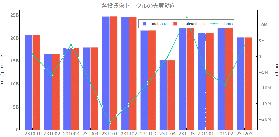
4-2. 委託売買の法人、個人、外国人投資家、証券会社の売買代金のtotal値の可視化
# グラフィック系ライブラリ
import plotly.graph_objects as go  # グラフ表示関連ライブラリ
import plotly.io as pio  # 入出力関連ライブラリ
pio.renderers.default = 'iframe'

# グラフの実体trace オブジェクトを生成
bar_trace_1 = go.Bar(x = df['date'], y = df['IndividualsTotal'], name = '個人')
bar_trace_2 = go.Bar(x = df['date'], y = df['ForeignersTotal'], name = '海外投資家')
bar_trace_3 = go.Bar(x = df['date'], y = df['SecuritiesCosTotal'], name = '証券会社')
bar_trace_4 = go.Bar(x = df['date'], y = df['InvestmentTrustsTotal'], name = '投資信託')
bar_trace_5 = go.Bar(x = df['date'], y = df['OtherCosTotal'], name = 'その他法人')
bar_trace_6 = go.Bar(x = df['date'], y = df['InsuranceCosTotal'], name = '生保・損保')
bar_trace_7 = go.Bar(x = df['date'], y = df['CityBKsRegionalBKsEtcTotal'], name = '都銀・地銀等')
bar_trace_8 = go.Bar(x = df['date'], y = df['TrustBanksTotal'], name = '信託銀行')
bar_trace_9 = go.Bar(x = df['date'], y = df['OtherFinancialInstitutionsTotal'], name = 'その他金融機関')

# レイアウトオブジェクトを生成
graph_layout = go.Layout(

    # 幅と高さの設定
    width=1000, height=600,

    # タイトルの設定
    title=dict(
        text='各投資家の売買動向', # タイトル
        font=dict(family='Times New Roman', size=20, color='grey'), # フォントの指定
        xref='paper', # container or paper
        x=0.5,
        y=0.87,
        xanchor='center',
    ),

    # y軸の設定
    yaxis=dict(
        # y軸のタイトルの設定
        title=dict(text='売買金額', font=dict(family='Times New Roman', size=20, color='grey')),
        # range=[0.0,6.0] # 軸の範囲の設定
    ),

    # 凡例の設定
    legend=dict(
        xanchor='left',
        yanchor='bottom',
        x=0.1,
        y=0.8,
        orientation='h',
        bgcolor='white',
        bordercolor='grey',
        borderwidth=1,
    ),
)

# 描画領域である figure オブジェクトの作成
fig = go.Figure(layout=graph_layout)

# add_trace()メソッドでグラフの実体を追加
fig.add_trace(bar_trace_1)
fig.add_trace(bar_trace_2)
fig.add_trace(bar_trace_3)
fig.add_trace(bar_trace_4)
fig.add_trace(bar_trace_5)
fig.add_trace(bar_trace_6)
fig.add_trace(bar_trace_7)
fig.add_trace(bar_trace_8)
fig.add_trace(bar_trace_9)

# レイアウトの更新
fig.update_layout(
    plot_bgcolor='white', # 背景色を白に設定
)

# 軸の設定
# linecolorを設定して、ラインをミラーリング(mirror=True)して枠にする
fig.update_xaxes(linecolor='black', linewidth=1, mirror=True)
fig.update_yaxes(linecolor='black', linewidth=1, mirror=True)

# ticks='inside':目盛り内側, tickcolor:目盛りの色, tickwidth:目盛りの幅、ticklen:目盛りの長さ
fig.update_xaxes(ticks='inside', tickcolor='black', tickwidth=1, ticklen=5)
fig.update_yaxes(ticks='inside', tickcolor='black', tickwidth=1, ticklen=5)

# gridcolor:グリッドの色, gridwidth:グリッドの幅、griddash='dot':破線
fig.update_xaxes(gridcolor='lightgrey', gridwidth=1, griddash='dot')
fig.update_yaxes(gridcolor='lightgrey', gridwidth=1, griddash='dot')

# 軸の文字サイズ変更
fig.update_xaxes(tickfont=dict(size=15, color='grey'))
fig.update_yaxes(tickfont=dict(size=15, color='grey'))

# show()メソッドでグラフを描画
fig.show()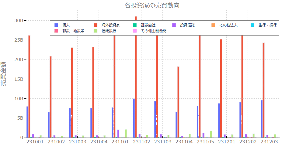
4-3. 海外投資家の売買動向の推移
# グラフィック系ライブラリ
import plotly.graph_objects as go  # グラフ表示関連ライブラリ
import plotly.io as pio  # 入出力関連ライブラリ
pio.renderers.default = 'iframe'

# グラフの実体trace オブジェクトを生成
bar_trace_1 = go.Bar(x = df['date'], y = df['ForeignersSales'], name = 'ForeignersSales',yaxis='y1')
bar_trace_2 = go.Bar(x = df['date'], y = df['ForeignersPurchases'], name = 'ForeignersPurchases',yaxis='y1')
scatter_trace_1 = go.Scatter(x = df['date'], y = df['ForeignersSales'] - df['ForeignersPurchases'] , name = 'balance',  yaxis='y2')

# レイアウトオブジェクトを生成
graph_layout = go.Layout(

    # 幅と高さの設定
    width=1000, height=600,

    # タイトルの設定
    title=dict(
        text='海外投資家の売買動向', # タイトル
        font=dict(family='Times New Roman', size=20, color='grey'), # フォントの指定
        xref='paper', # container or paper
        x=0.5,
        y=0.87,
        xanchor='center',
    ),

    # 軸の設定
    xaxis = dict(showgrid=False),
    yaxis = dict(title = 'sales / purchases', side = 'left', showgrid=False),
    yaxis2 = dict(title = 'balance', side = 'right',showgrid=False, overlaying = 'y'),

    # 凡例の設定
    legend=dict(
        xanchor='left',
        yanchor='bottom',
        x=0.5,
        y=0.85,
        orientation='h',
        bgcolor='white',
        bordercolor='grey',
        borderwidth=1,
    ),
)

# 描画領域である figure オブジェクトの作成
fig = go.Figure(layout=graph_layout)

# add_trace()メソッドでグラフの実体を追加
fig.add_trace(bar_trace_1)
fig.add_trace(bar_trace_2)
fig.add_trace(scatter_trace_1)

# レイアウトの更新
fig.update_layout(
    plot_bgcolor='white', # 背景色を白に設定
)

# 軸の設定
# linecolorを設定して、ラインをミラーリング(mirror=True)して枠にする
fig.update_xaxes(linecolor='black', linewidth=1, mirror=True)
fig.update_yaxes(linecolor='black', linewidth=1, mirror=True)

# ticks='inside':目盛り内側, tickcolor:目盛りの色, tickwidth:目盛りの幅、ticklen:目盛りの長さ
fig.update_xaxes(ticks='inside', tickcolor='black', tickwidth=1, ticklen=5)
fig.update_yaxes(ticks='inside', tickcolor='black', tickwidth=1, ticklen=5)

# gridcolor:グリッドの色, gridwidth:グリッドの幅、griddash='dot':破線
fig.update_xaxes(gridcolor='lightgrey', gridwidth=1, griddash='dot')
fig.update_yaxes(gridcolor='lightgrey', gridwidth=1, griddash='dot')

# 軸の文字サイズ変更
fig.update_xaxes(tickfont=dict(size=15, color='grey'))
fig.update_yaxes(tickfont=dict(size=15, color='grey'))

# show()メソッドでグラフを描画
fig.show()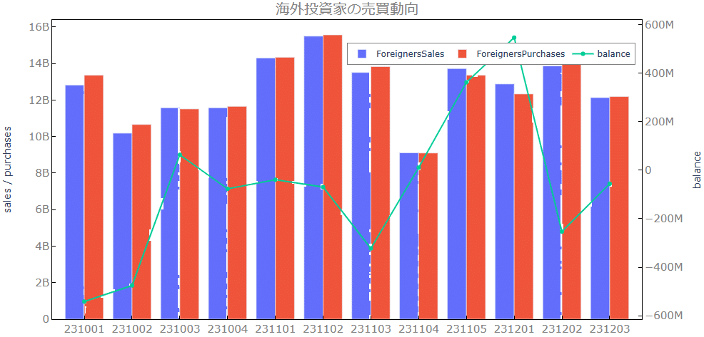
4-4. 個人投資家の売買動向の推移
# グラフィック系ライブラリ
import plotly.graph_objects as go  # グラフ表示関連ライブラリ
import plotly.io as pio  # 入出力関連ライブラリ
pio.renderers.default = 'iframe'

# グラフの実体trace オブジェクトを生成
bar_trace_1 = go.Bar(x = df['date'], y = df['IndividualsSales'], name = 'IndividualsSales',yaxis='y1')
bar_trace_2 = go.Bar(x = df['date'], y = df['IndividualsPurchases'], name = 'IndividualsPurchases',yaxis='y1')
scatter_trace_1 = go.Scatter(x = df['date'], y = df['IndividualsSales'] - df['IndividualsPurchases'] , name = 'balance',  yaxis='y2')

# レイアウトオブジェクトを生成
graph_layout = go.Layout(

    # 幅と高さの設定
    width=1000, height=600,

    # タイトルの設定
    title=dict(
        text='個人投資家の売買動向', # タイトル
        font=dict(family='Times New Roman', size=20, color='grey'), # フォントの指定
        xref='paper', # container or paper
        x=0.5,
        y=0.87,
        xanchor='center',
    ),

    # 軸の設定
    xaxis = dict(showgrid=False),
    yaxis = dict(title = 'sales / purchases', side = 'left', showgrid=False),
    yaxis2 = dict(title = 'balance', side = 'right',showgrid=False, overlaying = 'y'),

    # 凡例の設定
    legend=dict(
        xanchor='left',
        yanchor='bottom',
        x=0.5,
        y=0.85,
        orientation='h',
        bgcolor='white',
        bordercolor='grey',
        borderwidth=1,
    ),
)

# 描画領域である figure オブジェクトの作成
fig = go.Figure(layout=graph_layout)

# add_trace()メソッドでグラフの実体を追加
fig.add_trace(bar_trace_1)
fig.add_trace(bar_trace_2)
fig.add_trace(scatter_trace_1)

# レイアウトの更新
fig.update_layout(
    plot_bgcolor='white', # 背景色を白に設定
)

# 軸の設定
# linecolorを設定して、ラインをミラーリング(mirror=True)して枠にする
fig.update_xaxes(linecolor='black', linewidth=1, mirror=True)
fig.update_yaxes(linecolor='black', linewidth=1, mirror=True)

# ticks='inside':目盛り内側, tickcolor:目盛りの色, tickwidth:目盛りの幅、ticklen:目盛りの長さ
fig.update_xaxes(ticks='inside', tickcolor='black', tickwidth=1, ticklen=5)
fig.update_yaxes(ticks='inside', tickcolor='black', tickwidth=1, ticklen=5)

# gridcolor:グリッドの色, gridwidth:グリッドの幅、griddash='dot':破線
fig.update_xaxes(gridcolor='lightgrey', gridwidth=1, griddash='dot')
fig.update_yaxes(gridcolor='lightgrey', gridwidth=1, griddash='dot')

# 軸の文字サイズ変更
fig.update_xaxes(tickfont=dict(size=15, color='grey'))
fig.update_yaxes(tickfont=dict(size=15, color='grey'))

# show()メソッドでグラフを描画
fig.show()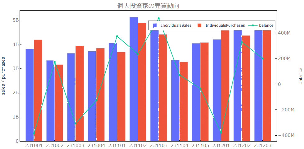
今回は、投資部門別の売買状況をJPX(日本取引所グループ)の投資部門別売買状況ページからデータをダウンロードして、plotlyで可視化して確認する方法を学びました。今後、2024年1月からの新NISA制度により、日本の個人投資家の投資売買がどう変化するかなども調査していきたいと思います。
この記事が気に入ったらサポートをしてみませんか?