VIX vs. NFCI = SPX weekly

ソース

TERM <- "2011::2022-11"
FC <- ANFCI
w <- merge(diff(apply.weekly(FC,mean))[TERM],as.vector(diff(apply.weekly(VIX[,4],mean))[TERM]))

colnames(w) <- c("FC","vix")
w <- merge(w,spx=as.vector(weeklyReturn(GSPC)[TERM]))
# w <- data.frame(w,s=cut(w$spx,breaks=c(min(w$spx),-0.025,0,0.025,max(w$spx)),labels=c('d','c','b','a'),include.lowest = T))
w <- data.frame(w,s=cut(w$spx,breaks=c(max(w$spx),0.01,0,-0.01,min(w$spx)),labels=c('a','b','c','d'),include.lowest = T))
# w$s <- factor(w$s,levels=c('a','b','c','d'))
w$s <- factor(w$s,levels=c('d','c','b','a')) # this is critical. never remove nor comment out.

df <- w
p <- ggplot(df, aes(x=FC,y=vix,color=s))
p <- p + geom_point(alpha=0.9)
# p <- p + guide_legend(reverse = TRUE)
# p <- p + scale_color_gradient(low = "green", high = "blue",name = "vix")
# p  <- p + scale_color_gradient2( low = "#FF0000",mid="#FFFF00" , high = "#0000FF",midpoint=0)
# p <- p + scale_color_discrete(name='spx daily return',label=c('less than -0.025','between -0.025 and 0','between 0 and 0.025','more than 0.025'))
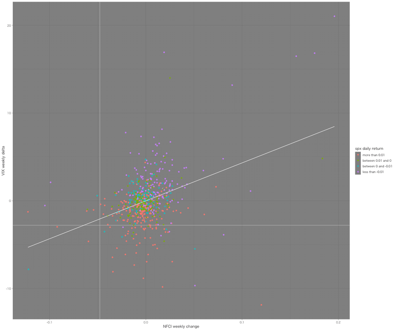
p <- p + scale_color_discrete(name='spx weekly return',label=c('more than 0.01','between 0.01 and 0','between 0 and -0.01','less than -0.01'))
p <- p + theme_dark(base_family = "HiraKakuPro-W3")
p <- p + stat_smooth(method = lm, formula = y ~ x,se=F,size=0.5,color='white')
p <- p + geom_vline(xintercept=(diff(apply.weekly(FC,mean)) %>% last()), colour="white",size=0.4,alpha=0.5)
p <- p + geom_hline(yintercept=(diff(apply.weekly(VIX[,4],mean)) %>% last()), colour="white",size=0.4,alpha=0.5)
p <- p + xlab("Financial Condition weekly change") + ylab("VIX weekly delta")   
plot(p)

回帰分析

summary(lm(w$spx ~ w$vix + w$FC))

Call:
lm(formula = w$spx ~ w$vix + w$NFCI)

Residuals:
      Min        1Q    Median        3Q       Max 
-0.065577 -0.008180  0.000059  0.008561  0.078221 

Coefficients:
              Estimate Std. Error t value Pr(>|t|)    
(Intercept)  0.0022440  0.0006941   3.233 0.001291 ** 
w$vix       -0.0049193  0.0002621 -18.768  < 2e-16 ***
w$NFCI      -0.0985548  0.0296093  -3.329 0.000925 ***
---
Signif. codes:  0 ‘***’ 0.001 ‘**’ 0.01 ‘*’ 0.05 ‘.’ 0.1 ‘ ’ 1

Residual standard error: 0.01724 on 614 degrees of freedom
Multiple R-squared:  0.4397,	Adjusted R-squared:  0.4379 
F-statistic: 240.9 on 2 and 614 DF,  p-value: < 2.2e-16

出力

ソースコード　拡張版

TERM <- "2011::2022-11"
FC <- ANFCI
w <- merge(diff(apply.weekly(FC,mean))[TERM],as.vector(diff(apply.weekly(VIX[,4],mean))[TERM]))

colnames(w) <- c("FC","vix")
w <- merge(w,spx=as.vector(weeklyReturn(GSPC)[TERM]))
# w <- data.frame(w,s=cut(w$spx,breaks=c(min(w$spx),-0.025,0,0.025,max(w$spx)),labels=c('d','c','b','a'),include.lowest = T))
w <- data.frame(w,s=cut(w$spx,breaks=c(max(w$spx),0.02,0.01,0,-0.01,-0.02,min(w$spx)),labels=c('a','b','c','d','e','f'),include.lowest = T))
# w$s <- factor(w$s,levels=c('a','b','c','d'))
w$s <- factor(w$s,levels=c('f','e','d','c','b','a')) # this is critical. never remove nor comment out.

df <- w
p <- ggplot(df, aes(x=FC,y=vix,color=s))
p <- p + geom_point(alpha=0.9,size=2)
# p <- p + guide_legend(reverse = TRUE)
# p <- p + scale_color_gradient(low = "green", high = "blue",name = "vix")
# p  <- p + scale_color_gradient2( low = "#FF0000",mid="#FFFF00" , high = "#0000FF",midpoint=0)
# p <- p + scale_color_discrete(name='spx daily return',label=c('less than -0.025','between -0.025 and 0','between 0 and 0.025','more than 0.025'))
# p <- p + scale_color_discrete(name='spx weekly return',label=c('more than 0.02','more than 0.01','between 0.01 and 0','between 0 and -0.01','less than -0.01','less than -0.02'))

p <- p + scale_color_brewer(name='spx weekly return',label=c('more than 0.02','more than 0.01','between 0.01 and 0','between 0 and -0.01','less than -0.01','less than -0.02'),palette='Spectral')
p <- p + theme_dark(base_family = "HiraKakuPro-W3")
p <- p + stat_smooth(method = lm, formula = y ~ x,se=F,size=0.5,color='white')
p <- p + geom_vline(xintercept=(diff(apply.weekly(FC,mean)) %>% last()), colour="white",size=0.4,alpha=0.5)
p <- p + geom_hline(yintercept=(diff(apply.weekly(VIX[,4],mean)) %>% last()), colour="white",size=0.4,alpha=0.5)
p <- p + xlab("Financial Condition weekly change") + ylab("VIX weekly delta")   
plot(p)