資金600万から資産1億円に到達する方法(その３、ランダムウォークから幾何ブラウン運動へ）

2024年2月18日 09:24

「600万円貯金があるけどどうしたら良いかな？1億円目指してFIREしたいんだけど。やっぱ個別株をタイミング見て買うのが良いかな？」、若い友人と相談を受けました。「うーん、どうかな、その方法だと資金を全部溶かす可能性が高いです」と返事をしました。その質問をきっかけに一般投資家にとって最適な株式の投資戦略はなんでしょう？というのを考えてみます。ここまでのメッセージをまとめると下記のようになります。

勝率の期待値が50％を超える投資をする、50％を下回る投資はしない
勝率が高い場合でも1回の投資額を増やすと破産する可能性が高まる
どんなに良い投資でも初期の元本割れは許容しないといけない
元本割れした場合はしばらく元本割れの期間が続くことが多いが投資は中断してはいけない

これまではコイントスをモデルに検証しましたが実際の投資での株価の動きは”幾何ブラウン運動”がモデルとしてよく使われます。。単純なコイントスでのランダムウォークから幾何ブラウン運動の方程式を導きその特徴を検討してみます。またこのブログ記事では実際にPythonのコードを書いて実行しながら理解していくことを目標にしています。

ランダムウォーク

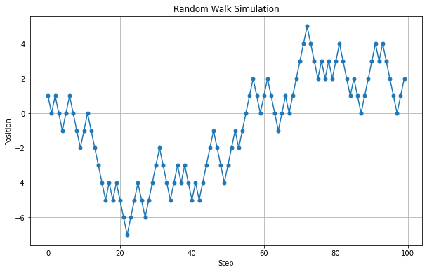
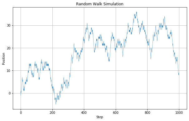
まずコイントスによるランダムウォークを考えます。50%の確率で＋１、50%の可能性で-1進みます、それを100回繰り返した際の位置をグラフにしてみます。

import numpy as np
import matplotlib.pyplot as plt

# Set the seed for reproducibility
np.random.seed(0)

# Define the number of steps
n_steps = 100

# Simulate the steps: +1 or -1 with equal probability
steps = np.random.choice([-1, 1], size=n_steps)
position = np.cumsum(steps)  # Cumulative sum to get the position

# Plot the position over time
plt.figure(figsize=(10, 6))
plt.plot(position, marker='o', linestyle='-', markersize=5)
plt.title('Random Walk Simulation')
plt.xlabel('Step')
plt.ylabel('Position')
plt.grid(True)

# Show the plot
plt.show()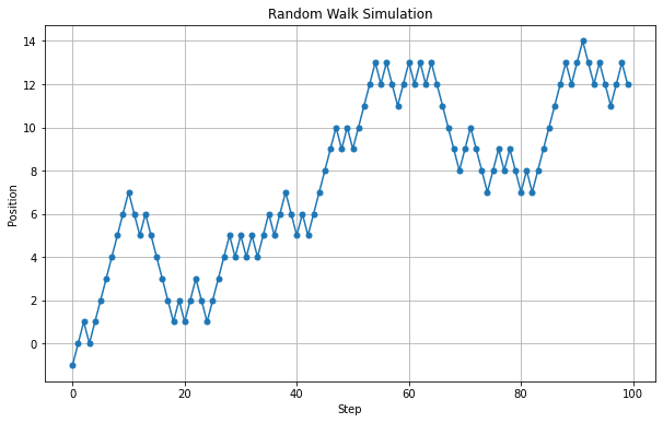

上記のコードでは再現性を持たせるために下記コードを入れています。

# Set the seed for reproducibility
np.random.seed(0)

毎回違うグラフを出力したい場合はこの部分を削除します。そうすると毎回違うグラフが出力されます。

株価のチャートににていますね。これを100回繰り返して重ね合わせるとどうなるでしょう？

# Define the number of simulations
n_simulations = 100

# Initialize an array to hold the final positions for each simulation
final_positions = np.zeros((n_simulations, n_steps))

# Perform the simulations
for i in range(n_simulations):
    steps = np.random.choice([-1, 1], size=n_steps)
    final_positions[i] = np.cumsum(steps)

# Plot the positions for all simulations
plt.figure(figsize=(10, 6))
for i in range(n_simulations):
    plt.plot(final_positions[i], alpha=0.5)  # Reduced opacity to see overlapping paths

plt.title('Random Walk Simulation Overlaid 100 Times')
plt.xlabel('Step')
plt.ylabel('Position')
plt.grid(True)

# Show the plot
plt.show()

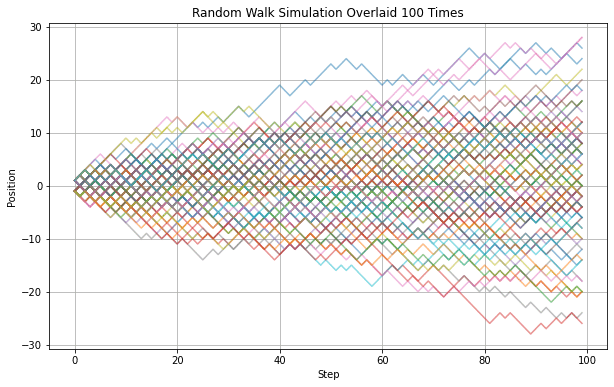
　100回繰り返すと理論的には‐100～＋100まで最終的な位置は分布します。分布をヒストグラムで表してみます。

# Extract the final position from each simulation
final_positions_last_step = final_positions[:, -1]

# Plot the histogram of the final positions
plt.figure(figsize=(10, 6))
plt.hist(final_positions_last_step, bins=20, alpha=0.7)
plt.title('Histogram of Final Positions After 100 Steps')
plt.xlabel('Final Position')
plt.ylabel('Frequency')
plt.grid(True)

# Show the plot
plt.show()

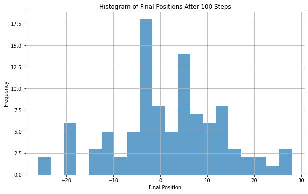
分布は0を中心に分布しているようですが100回ですとばらつきが大きいので1,000,000回に増やしてみます。そしてヒストグラムをランダムウォークの推移のグラフと並べてみます。

import numpy as np
import matplotlib.pyplot as plt
from matplotlib import gridspec

# Define the number of steps and simulations
n_steps = 100
n_simulations = 1000000
n_subset_simulations = 100  # Number of paths to actually plot for clarity

# Initialize an array to hold the final positions for each simulation in the subset
np.random.seed(0)  # Ensure reproducibility
final_positions_subset = np.zeros((n_subset_simulations, n_steps))

# Perform the subset of simulations
for i in range(n_subset_simulations):
    steps = np.random.choice([-1, 1], size=n_steps)
    final_positions_subset[i] = np.cumsum(steps)

# Simulate final positions for 1,000,000 random walks using normal approximation
final_positions_last_step_full = np.random.normal(0, np.sqrt(n_steps), n_simulations)

# Create figure and gridspec for custom subplot sizes
fig = plt.figure(figsize=(16, 6))
gs = gridspec.GridSpec(1, 3)  # 1 row, 3 columns grid

# Plot the representative subset of random walk paths in the first two columns
ax1 = plt.subplot(gs[0, 0:2])
for i in range(n_subset_simulations):
    ax1.plot(final_positions_subset[i], alpha=0.5)
ax1.set_title('Representative Random Walk Paths')
ax1.set_xlabel('Step')
ax1.set_ylabel('Position')
ax1.grid(True)

# Plot the histogram of final positions in the third column, with horizontal orientation and flipped
ax2 = plt.subplot(gs[0, 2])
ax2.hist(final_positions_last_step_full, bins=40, alpha=0.7, orientation='horizontal', color='red', density=True)
ax2.set_title('Distribution (Flipped)')
ax2.set_xlabel('Density')
ax2.set_ylabel('Position')
ax2.grid(True)
ax2.invert_xaxis()  # Flip the histogram horizontally

plt.tight_layout()
plt.show()

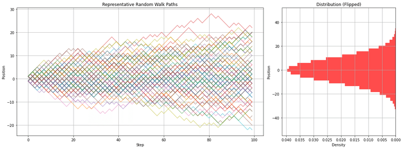
こうすると最終的な位置の分布が0を中心に±対象に分布していることがわかると思います（代表的な100回のパスを折れ線グラフで表示）。このシミュレーションの最終的な位置の平均（期待値）は0ですし、分散は100になります。実際にプログラムを書いて計算してみます。

# Calculate and print the mean and variance of the final positions
mean_position = np.mean(final_positions_last_step_full)
variance_position = np.var(final_positions_last_step_full)

print(f"Mean of final positions: {mean_position}")
print(f"Variance of final positions: {variance_position}")

ランダムウォークの最終的な位置の統計量は以下の通りです：

平均（Mean）: 0
分散（Variance）: 100

ステップが100の場合に分散が100、では1000のステップで同じ計算をしてみます。先程のステップ数を1000に変更するだけです。

import numpy as np
import matplotlib.pyplot as plt
from matplotlib import gridspec

# Define the number of steps and simulations
n_steps = 1000
n_simulations = 1000000
n_subset_simulations = 100  # Number of paths to actually plot for clarity

# Initialize an array to hold the final positions for each simulation in the subset
np.random.seed(0)  # Ensure reproducibility
final_positions_subset = np.zeros((n_subset_simulations, n_steps))

# Perform the subset of simulations
for i in range(n_subset_simulations):
    steps = np.random.choice([-1, 1], size=n_steps)
    final_positions_subset[i] = np.cumsum(steps)

# Simulate final positions for 1,000,000 random walks using normal approximation
final_positions_last_step_full = np.random.normal(0, np.sqrt(n_steps), n_simulations)

# Create figure and gridspec for custom subplot sizes
fig = plt.figure(figsize=(16, 6))
gs = gridspec.GridSpec(1, 3)  # 1 row, 3 columns grid

# Plot the representative subset of random walk paths in the first two columns
ax1 = plt.subplot(gs[0, 0:2])
for i in range(n_subset_simulations):
    ax1.plot(final_positions_subset[i], alpha=0.5)
ax1.set_title('Representative Random Walk Paths')
ax1.set_xlabel('Step')
ax1.set_ylabel('Position')
ax1.grid(True)

# Plot the histogram of final positions in the third column, with horizontal orientation and flipped
ax2 = plt.subplot(gs[0, 2])
ax2.hist(final_positions_last_step_full, bins=40, alpha=0.7, orientation='horizontal', color='red', density=True)
ax2.set_title('Distribution (Flipped)')
ax2.set_xlabel('Density')
ax2.set_ylabel('Position')
ax2.grid(True)
ax2.invert_xaxis()  # Flip the histogram horizontally

plt.tight_layout()
plt.show()
# Calculate and print the mean and variance of the final positions
mean_position = np.mean(final_positions_last_step_full)
variance_position = np.var(final_positions_last_step_full)

print(f"Mean of final positions: {mean_position}")
print(f"Variance of final positions: {variance_position}")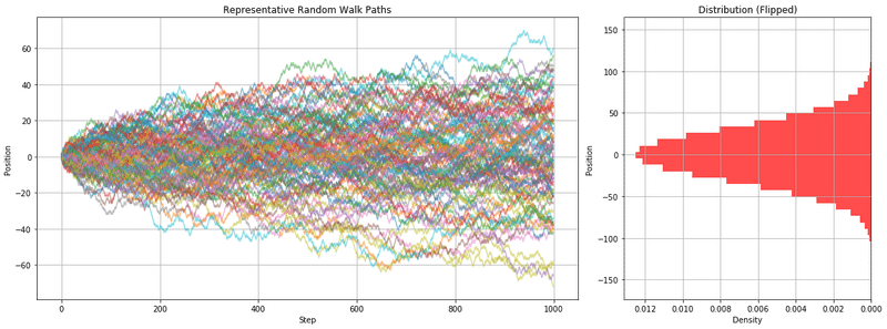

平均（Mean）: 0
分散（Variance）: 1000

となります。そうするとステップ数を増やしても平均は0のまま、分散はステップ数に一致することがわかります。つまりコイントスでのランダムウォークの場合はステップ数が増えるたびに分散が増える（散らばりがおおきくなる）ことがわかります。実際にステップ数を10、100、1000と増やした場合のヒストグラムがどうなるか確認してみます。

import numpy as np
import matplotlib.pyplot as plt
from matplotlib import gridspec

# Define the number of steps for the simulations
steps_list = [10, 100, 1000]
n_simulations = 100000

# Create figure and gridspec for custom subplot sizes
fig = plt.figure(figsize=(18, 6))
gs = gridspec.GridSpec(1, 3)  # 1 row, 3 columns grid

# Find global min and max for the positions to unify axis scales
all_positions = []
for n_steps in steps_list:
    all_positions.extend(np.random.normal(0, np.sqrt(n_steps), n_simulations))
global_min = min(all_positions)
global_max = max(all_positions)

# Find the maximum density to unify x-axis (density) scale across all histograms
max_density = 0
for n_steps in steps_list:
    counts, bin_edges = np.histogram(np.random.normal(0, np.sqrt(n_steps), n_simulations), bins=40, density=True)
    max_density = max(max_density, max(counts))

# Loop over the steps_list to generate flipped horizontal histograms for each step count
for index, n_steps in enumerate(steps_list):
    # Simulate final positions again for consistency
    final_positions_last_step = np.random.normal(0, np.sqrt(n_steps), n_simulations)
    
    # Plot the histogram of final positions in the respective column
    ax = plt.subplot(gs[0, index])
    ax.hist(final_positions_last_step, bins=40, alpha=0.7, orientation='horizontal', color='red', density=True)
    ax.set_title(f'{n_steps} Steps')
    ax.set_xlabel('Density')
    ax.set_ylabel('Position')
    ax.grid(True)
    ax.set_xlim(0, max_density)  # Unify x-axis (density) scale across all plots
    ax.invert_xaxis()  # Flip the histogram horizontally
    ax.set_ylim(global_min, global_max)  # Keep y-axis scale unified

# Adjust layout to prevent overlap
plt.tight_layout()
plt.show()

# Calculate and print the mean and variance of the final positions for each step count

results = {}  # Dictionary to store results

for n_steps in steps_list:
    # Simulate final positions for 100,000 random walks
    final_positions = np.random.normal(0, np.sqrt(n_steps), n_simulations)
    
    # Calculate mean and variance
    mean_position = np.mean(final_positions)
    variance_position = np.var(final_positions)
    
    # Store results
    results[n_steps] = {'Mean': mean_position, 'Variance': variance_position}

results

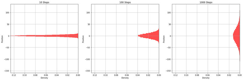
いずれの場合も期待値は0ですが分散は10、100、1000と増加していくことがわかります。

ランダムウォークの平均と分散

コイントスの一回の移動量をσで表し一般化すると下記が成り立ちます。

一回の移動量（ステップサイズ）をσで表す場合、ランダムウォークの各ステップの移動量の分散は$${\sigma^2}$$ と表されます。ここで、σは各ステップにおける移動量の標準偏差とも言えます。ステップ数をtで表します。

ランダムウォークにおける一歩の平均は以下のように表されます。

$$
E[\Delta r(t)] = 0
$$

一歩の移動量の分散 $${\sigma^2}$$は、ランダムウォークにおける一歩の分散も同様に $${\sigma^2}$$であることを意味します。

$$
V[\Delta r(t)] = \sigma^2
$$

tステップ後の平均位置の変化は、依然として 0 です。

$$
E[r(t)] = 0
$$

tステップ後の分散は、各ステップが独立しているため、t倍の$${\sigma^2}$$ に等しくなります。

$$
V[r(t)] = t\sigma^2
$$

これは、ランダムウォークにおける各ステップの移動量が一定の標準偏差 σを持つ場合に適用され、ステップ数 t が増加するにつれて最終的な位置の分散も増加することを示します。先程の例ですとσ=1ですから100ステップ後の分散は100ですし、1000ステップ後の分散は1000です。なお、平均はいずれも0です。

ランダムウォークをそのまま株式シミュレーションに用いる場合もありますが、グラフを見てみますと

株価の推移と考えるにはギザギザとしすぎてみます。ステップ数を細かくしていけば株価の変動に近づいていきそうです。例えばステップ数を1000にしてみます。

と株価のチャートに似てきます。このような完全にランダムに作成されたチャートでも色付けをして25日移動平均線、75日移動平均線を書き込むと下記のようになりテクニカル分析は可能です。

import numpy as np
import matplotlib.pyplot as plt


# Define the number of steps
n_steps = 1000

# Simulate the steps: +1 or -1 with equal probability
steps = np.random.choice([-1, 1], size=n_steps)
position = np.cumsum(steps)  # Cumulative sum to get the position

# Calculate moving averages
moving_avg_25 = np.convolve(position, np.ones(25)/25, mode='valid')
moving_avg_75 = np.convolve(position, np.ones(75)/75, mode='valid')

# Plot the position over time
plt.figure(figsize=(10, 6))

# Plot position with color based on direction
for i in range(1, len(position)):
    if position[i] > position[i-1]:  # If the position has increased
        plt.plot([i-1, i], [position[i-1], position[i]], 'g-')  # Use green
    else:  # If the position has decreased or stayed the same
        plt.plot([i-1, i], [position[i-1], position[i]], 'r-')  # Use red

# Plot moving averages
plt.plot(np.arange(24, n_steps), moving_avg_25, 'm-', label='25-Day Moving Average')
plt.plot(np.arange(74, n_steps), moving_avg_75, 'k-', label='75-Day Moving Average')

plt.title('Random Walk Simulation with Moving Averages')
plt.xlabel('Step (Day)')
plt.ylabel('Position')
plt.legend()
plt.grid(True)

# Show the plot
plt.show()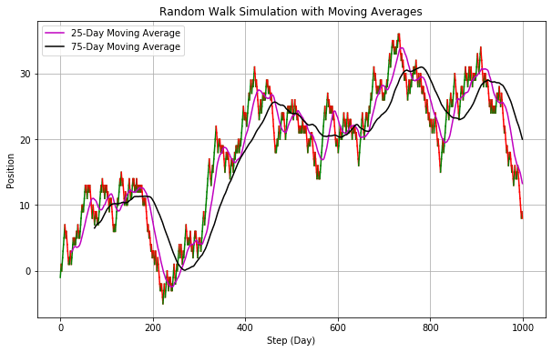

このチャートはランダムウォークなので移動平均線を引いてゴールデンクロス、デッドクロスといっても意味がありません。株価がランダムウォークであればテクニカル分析はまったく意味をなさないです。下記のチャートはいずれもランダムウォークにおり出力されたチャートです。

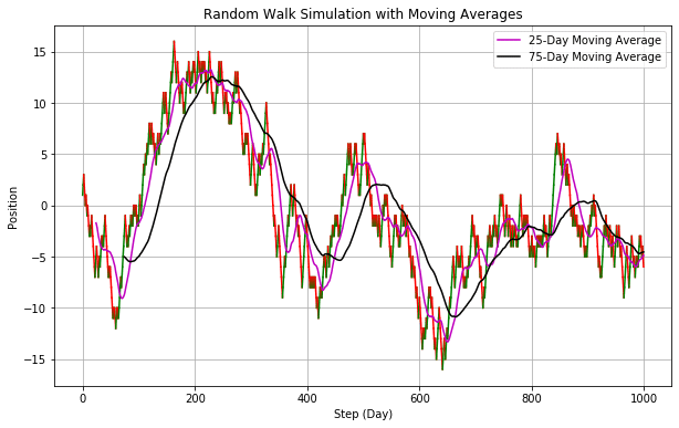
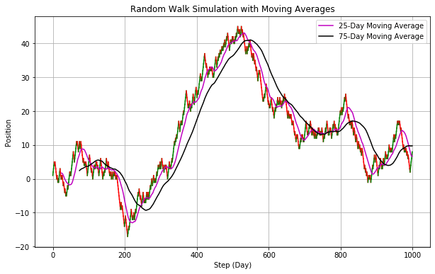
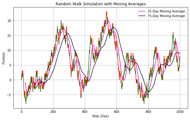
移動平均線を引くと一定の法則がありそうに見えますが移動の法則はありません。これを株価のチャートだとするとここで買って、ここで売って、みたいに考えてしまいそうになりますが移動平均線から売り買いのタイミングを考えてもまったく意味がないです。さらに言えば、株の売り買いには売買手数料がかかりますから何も考えずに最初に買って持っている人よりも期待値は下がります。このことから”あなたが株価がランダムウォークと考えるのであればテクニカル分析や売り買いのタイミングを考えることは無意味かつ有害である”ということが言えます。

ランダムウォークから幾何ブラウン運動へ

ランダムウォークでも株価のシミュレーションは可能ですがステップごとに株価の移動距離がきまっているので、これを更に微小な変化に変化させると考えると株価のシミュレーションで用いられる幾何ブラウン運動の式になります。また株価は一定の傾向、通常は増加する傾向があるため”幾何”ブラウン運動となりますが疲れたのでまた次回に。

この記事が気に入ったらサポートをしてみませんか？