Data Analysis with Python (quick note)

1. Importing Datasets

You can download my .ipynb here: 

DataAnalysis_Week1.ipynb

117 KB

ファイルダウンロードについて

ダウンロード

Formats for dataset: .csv, .json, .xls
Pandas Library: 
- Read datasets into a data frame

# import pandas as pd
import pandas as pd

Read data:

path = "path of the data file (it can be a link or a file in the computer)"
df = pd.read_csv(other_path, header=None)

df.head(n)
df.tail(n)
# check the top n rows / bottom n rows of the dataframe

Add header:

# create headers list
headers = ["abc","efg","xyz"]

# replace headers
df.columns = headers

Drop missing values:

df.dropna(subset=["name of column want to drop"], axis = 0)

Save Dataset:

df.to_csv("file_name.csv", index = False)

Data Types:
- object
- float
- int
- bool
- datetime64

# print the type of each column
df.dtypes

Describe:
- Get a statistical summary of each column (count, mean, SD)

df.describe() # excluding NaN (Not a Number)
df.describe(include = "all") # including NaN

# apply describe for selected columns
df[["column1","column2","column3"]].describe()

Info:
- Provide a concise summary of DataFrame

df.info

2. Data Wrangling

You can download my .ipynb here: 

DataAnalysis_Week2.ipynb

110 KB

ファイルダウンロードについて

ダウンロード

Data Pre-processing: converting/mapping data from "raw" form into another format
Data Cleaning / Data Wrangling
Learning Objectives:
- Identify and handle missing values
- Data Formatting
- Data Normalization (centering/scaling)
- Data Binning
- Turning Categorical values to numeric variables

Missing values: "?", "N/A", 0 or a blank cell
How to deal with missing data?
- Drop the missing values: variable / data entry
- Replace the missing values with: an average, frequency, based on other functions
- Leave it as missing data

Drop:

df.dropna()
# axis = 0: drops the entire row
# axis = 1: drops the entire column
df.dropna(subnet = ["column want to drop"],axis = 0, inplace = True)

Python Data Analysis Library — pandas: Python Data Analysis Library

Replace:

df.replace(missing_value, new_value)
df["column"].replace(np.nan, mean)

Data Formatting: bringing data into a common standard of expression

df["column"] = n / df["column"] # convert data by a formula
# rename columns
df.rename(columns={"column":"another_name"}, inplace = True)

Correcting data types

# identify data type
df.dtypes()
# convert data type
df.astype()
df["column"] = df["column"].astype("int")

Data Normalization: convert to the similar value range / similar intrinsic influence on analytical model
3 ways:
- Simple Feature scaling: xnew = xold / xmax
- Min-Max: xnew = (xold - xmin) / (xmax - xmin)
- Z-score (standard score): xnew = (xold - u) / o (u: mean, o: SD)

df["col"] = df["col"] / df["col"].max()
df["col"] = (df["col"] - df["col"].min()) / (df["col"].max() - df["col"].min())
df["col"] = (df["col"] - df["col"].mean()) / (df["col"].std())

Binning:
- Binning: Grouping of values into "bins"
- Converts numeric into categorical variables
- Group a set of numerical values into a set of "bins"

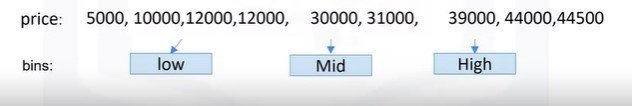
bins = np.linspace(min(df["col"]), max(df["col"]), 4)
group_names = ["Low", "Medium", "High"]
df["col-binned"] = pd.cut(df["col"], bins, labels = group_names, include_lowest = True)

Turning categorical variables into quantitative variables in Python
Categorical -> Numeric:
- Add dummy variables for each unique category
- Assign 0 or 1 in each category
One-hot encoding

pd.get_dummies(df['fuel'])

3. Exploratory Data Analysis (EDA)

You can download my .ipynb here: 

DataAnalysis_Week3.ipynb

245 KB

ファイルダウンロードについて

ダウンロード

Descriptive Statistics
GroupBy
ANOVA
Correlation
Correlation - Statistics

Descriptive Statistics:
- Describe basic features of data
- Giving short summaries about the sample and measures of the data

df.describe()
data_counts = df["column"].value_counts()
data_counts.rename(columns={'old_name':'new_name',inplace = True)
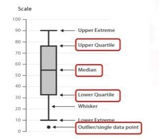
data_counts.index.name = 'old_name'

Box Plot

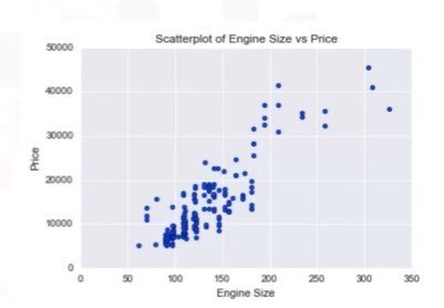
Scatter Plot:
- Each observation represented as a point
- Scatter plot shows the relationship between two variables
- Predictor / independent variables on x-axis
- Target / dependent variables on y-axis

GroupBy:
- Can be applied on categorical variables
- Group data into categories

df_test = df['column1', 'column2', 'column3']
df_grp = df_test.groupby(['column1', 'column2'], as_index=False).mean()
df_grp

GroupBy Pivot()

df_pivot = df_grp.pivot(index = 'column1', columns = 'column2')

Heatmap

plt.pcolor(df_pivot,cmap='RdBBu')
plt.colorbar()
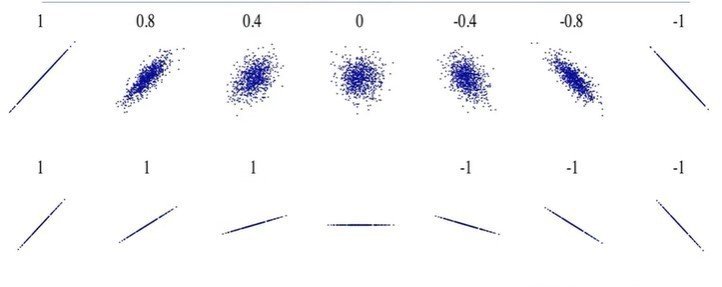
plt.show()

Correlation:
- Positive Linear Relationship
- Negative Linear Relationship
- Strong and Weak correlation

sns.regplot(x="x-name", y="y-name", data = df)
plt.ylim(0,)

Pearson Correlation:
Correlation coefficient:
- Close to +1: Large Positive relationship
- Close to -1: Large Negative relationship
- Close to 0: No relationship
P-value
<0.001: Strong certainly in the result
<0.05: Moderate certainly in the result
<0.1: Weak certainly in the result
>0.1: No certainly in the result
Strong Correlation:
- Correlation coefficient close to 1 or -1
- P-value less than 0.001

Pearson_coef, p_value = stats.personr[['column1'],df['column2']]

Analysis of Variance (ANOVA)
Statistical comparison of groups
Finding correlation between different groups of a categorical variable
ANOVA:
- F-test score: variation between sample group means divided by variation within sample group
- p-value: confidence degree

F-test:
- Small F: poor correlation between groups
- Large F: strong correlation between groups

# ANOVA between "Honda" and "Subaru"
df_anova = df[["make","price"]]
grouped_anova = df_anova.groupby(["make"])
anova_results_1 = stats.f_oneway(grouped_anova.get_group("honda")["price"], grouped_anova.get_group("subaru")["price"])

4. Model Development

You can download my .ipynb here: 

DataAnalysis_Week4.ipynb

251 KB

ファイルダウンロードについて

ダウンロード

Simple and Multiple Linear Regression
Model Evaluation using Visualization
Polynomial Regression and Pipelines
R-squared and MSE for In-Sample Evaluation
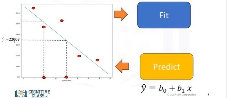
Prediction and Decision Making

Model:
- Independent variables
- Dependent variables
- Relevant data

Simple Linear Regression
- The predictor (independent): x
- The target (dependent): y
- The intercept: b0
- The slope: b1
- y = b0 + b1x
- (b0, b1): Fit

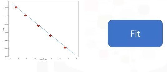
X = df[['x-axis-columns']]
Y = df[['y-axis-columns']]
lm.fit(X,Y)
Yhat = lm.predict(X)

Multiple Linear Regression (MLR)
_ One continuous target (Y) variable
- Two or more predictor (X) variables
- y = b0 + b1x1 + b2x2 + b3x3 + b4x4
- b0: intercept
- bn: coefficient or parameter of xn

Z = df[['x-axis-columns'],['y-axis-columns'],['z-axis-columns']]
lm.fit(Z,df['column'])
Yhat = lm.predict(X)

Estimated Linear Model:
- Find the intercept (b0)
- Find the coefficients (b1, b2, b3, b4)

Model Evaluation using Visualization:
Regression Plot:
- The relationship between two variables
- The strength of correlation
- The direction of the relationship (P or N)
- The scatterplot
- The fitted linear regression line

import seaborn as sns
sns.regplot(x="x-axis-column", y = "y-axis-column", data = df)
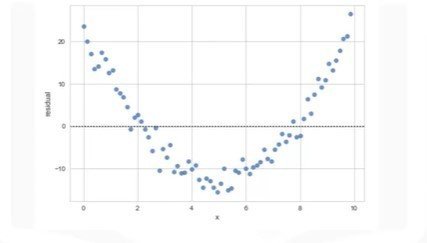
plt.ylim(0,)

Residual Plot
- Spread of the residuals: randomly spread out around x-axis

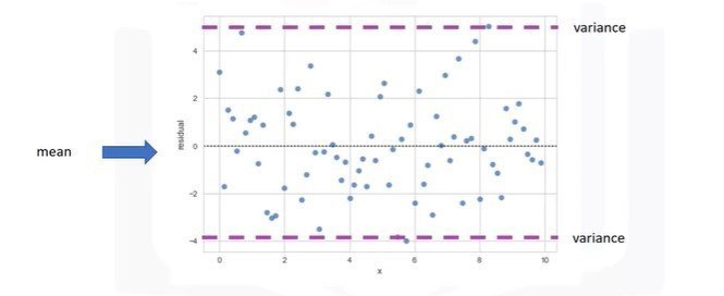
- Not randomly spread out around x-axis
- Nonlinear model may be more appropriate

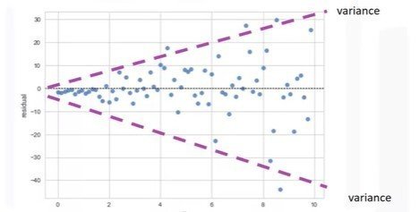
- Not randomly spread out around x-axis
- Variance appears to change with x-axis

import seaborn as sns
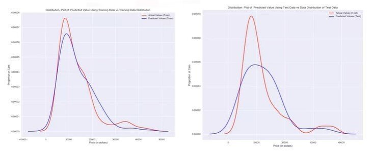
sns.residplot(df['x-axis-column'], df['y-axis'])

Distribution Plots
- The fitted values that result from the model
- The actual values

import seaborn as sns
ax1 = sns.distplot(df['column'], hist = False, color="r", label="Actual Value")
sns.distplot(Yhat, hist=False, color="b", label="Fitted Values", ax=ax1)

Polynomial Regression
- Quadratic - 2nd order: y = b0 + b1x1 + b2(x1)^2
- Cubic - 3rd order: y = b0 + b1x1 + b2(x1)^2 + b3(x1)^3

f = np.polyfit(x,y,3)
p = np.polydl(f)

One Dimension

from sklearn.preprocessing import PolynomialFeatures
pr = PolynomialFeatures(degree=2)
x_polly = pr.fit_transform(x['column1','column2'],include_bias = False)

Pre-processing

from sklearn.preprocessing import StandardScaler
SCALE = StandardScaler()
SCALE.fit(x_data[['column1'],['column2']])
x_scale = SCALE.transform(x_data[['column1'],['column2']])

Pipelines

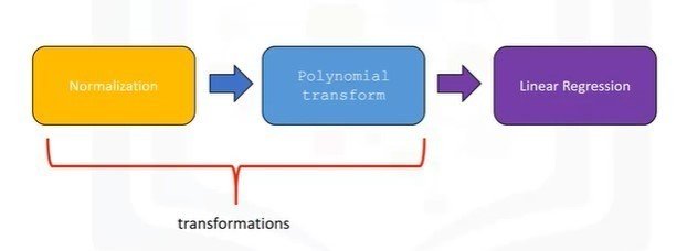
from sklearn.preprocessing import PolynomialFeatures
from sklearn.preprocessing import LinearRegression
from sklearn.preprocessing import StandardScaler

Pipeline Constructor

Pipe.train(X['column1'],['column2'],['column3'],['column4'])
yhat = Pipe.predict(X['column1'],['column2'],['column3'],['column4'])

Measures for In-Sample Evaluation
Numerically determine how good the model fits on dataset
Two important measures to determine the fit of a model:
- Mean Squared Error (MSE)
- R-squared (R^2)

Mean Squared Error (MSE)

from sklearn.metrics import mean_squared_error
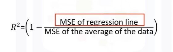
mean_squared_error(df['column'], Y_predict_simple_fit)

R-squared / R^2
- The coefficient of Determination or R squared (R^2)
- Determine how close the data is to the fitted regression line
- R^2: the percentage of variation of the target variable (Y) that is explained by the linear model

The values of MSE are between 0 and 1

X = df[['x-axis-column]]
Y = df['y-axis-column]
lm.fit(X,Y)
lm.score

Prediction and Decision Making
Determining a Good Model Fit:
- Do the predicted values make sense
- Visualization
- Numerical measures for evaluation
- Comparing Models

# Train the model
lm.fit(df['x-axis-column'],df['y-axis-column']]
lm.predict(x-value)
lm.coef_

import numpy as np
new_input = np.arange(1,101,1).reshape(-1,1)
# Predict new values
yhat = lm.predict(new_input)

Numerical measures of Evaluation
Compare MLR and SLR:
- MSE for MLR model will be smaller than MSE for SLR model
- Polynomial regression will also have smaller MSE
- A similar inverse relationship holds for R^2

5. Model Evaluation and Refinement

You can download my .ipynb here: 

Model Evaluation:
In-Sample evaluation: how well our model will fit the data used to train it
Out-of-sample evaluation or test set
Split data set into:
- training set: 70% - build and train the model
- testing set: 30% - assess the performance of a predictive model

from sklearn.model_selection import train_test_split
x_train, x_test, y_train, y_test = train_test_split(x_data, y_data, test_size = 0.3, random_state = 0)

x_data: features or independent variables
y_data: dataset target
x_train, y_train: parts of available data as training set
x_test, y_test: parts of available data as testing set
test_size = 30/100 = 0.3
random_state: number generator used for random sampling

Generalization Performance:
Generalization error: measure of how well data does at predicting previously unseen data