深層学習3dayレポート

Section1:再帰型ニューラルネットワークの概念
【解説】
1-1:RNN全体像
1RNNとは時系列データに対応可能な、ニューラルネットワーク。時系列データとは、時間的順序を追って一定間隔ごとに観察され、しかも相互に統計的依存関係が認められるようなデータの系。音声データ・テキストデータ...などが有る。
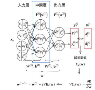
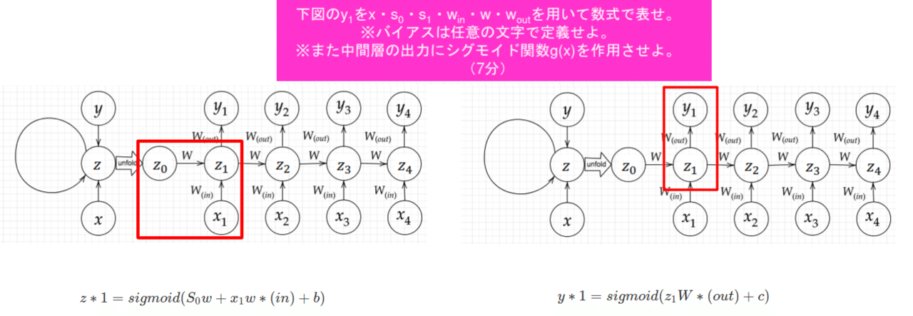
構造はニューラルネットワーク。ただ、Wが前の中間層からの重みも存在している。
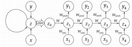
このような書き方をされる。
時系列モデルを扱うには、初期の状態と過去の時間t-1の状態を保持し、そこから次の時間でのtを再帰的に求める再帰構造が必要になる。
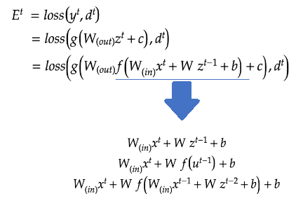
1-2:BPTT(Backpropagation Through Time)
リカレントニューラルネットワークの誤差を求める際に、時間軸で展開するイメージ。誤差が時間をさかのぼって逆伝播し誤差逆伝播の一種と言える。
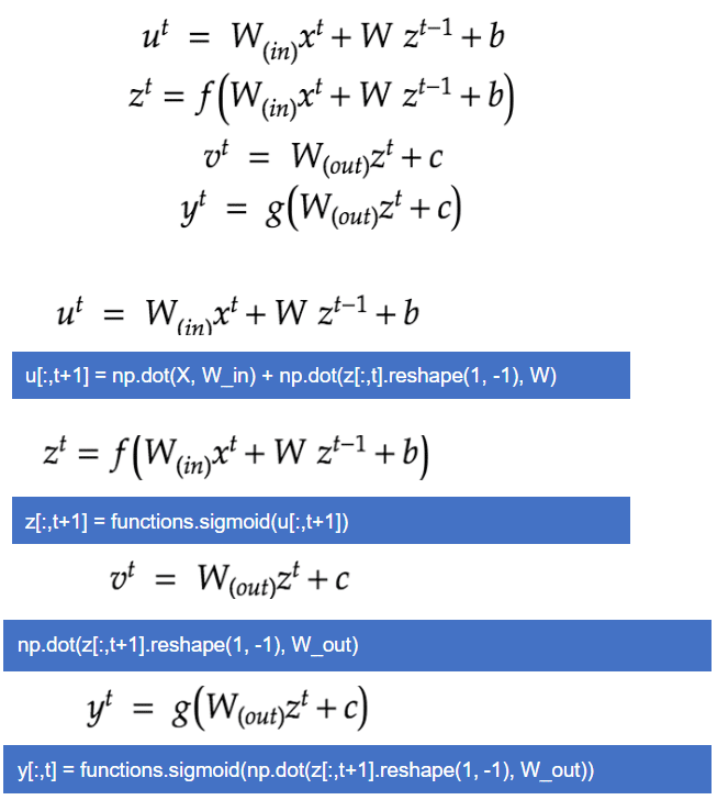
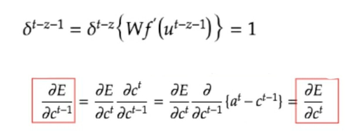
BPTTの数学記述1
BPTTの数学記述2
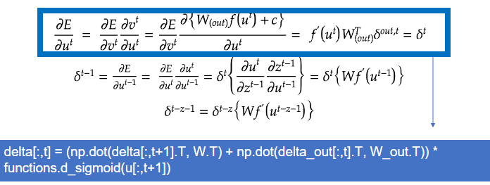
BPTTの数学記述3
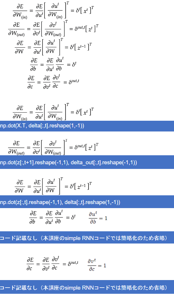
BPTTの数学記述4
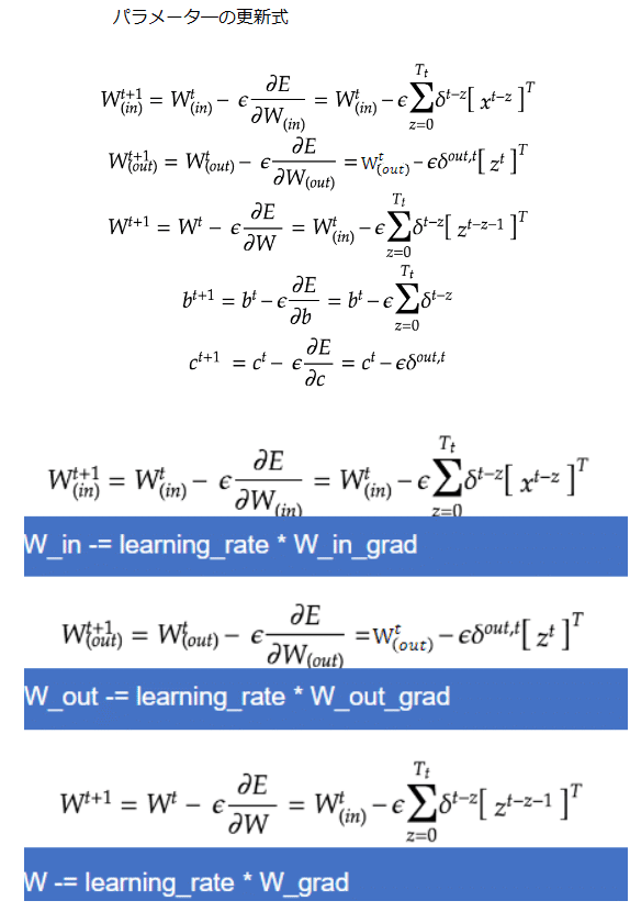
BPTTの全体像
【実装/演習】
import numpy as np
from common import functions
import matplotlib.pyplot as plt
# def d_tanh(x):
# データを用意
# 2進数の桁数
binary_dim = 8
# 最大値 + 1
largest_number = pow(2, binary_dim)
# largest_numberまで2進数を用意
binary = np.unpackbits(np.array([range(largest_number)],dtype=np.uint8).T,axis=1)
input_layer_size = 2
hidden_layer_size = 16
output_layer_size = 1
weight_init_std = 1
learning_rate = 0.1
iters_num = 10000
plot_interval = 100
# ウェイト初期化 (バイアスは簡単のため省略)
W_in = weight_init_std * np.random.randn(input_layer_size, hidden_layer_size)
W_out = weight_init_std * np.random.randn(hidden_layer_size, output_layer_size)
W = weight_init_std * np.random.randn(hidden_layer_size, hidden_layer_size)
# Xavier
# He
# 勾配
W_in_grad = np.zeros_like(W_in)
W_out_grad = np.zeros_like(W_out)
W_grad = np.zeros_like(W)
u = np.zeros((hidden_layer_size, binary_dim + 1))
z = np.zeros((hidden_layer_size, binary_dim + 1))
y = np.zeros((output_layer_size, binary_dim))
delta_out = np.zeros((output_layer_size, binary_dim))
delta = np.zeros((hidden_layer_size, binary_dim + 1))
all_losses = []
for i in range(iters_num):
# A, B初期化 (a + b = d)
a_int = np.random.randint(largest_number/2)
a_bin = binary[a_int] # binary encoding
b_int = np.random.randint(largest_number/2)
b_bin = binary[b_int] # binary encoding
# 正解データ
d_int = a_int + b_int
d_bin = binary[d_int]
# 出力バイナリ
out_bin = np.zeros_like(d_bin)
# 時系列全体の誤差
all_loss = 0
# 時系列ループ
for t in range(binary_dim):
# 入力値
X = np.array([a_bin[ - t - 1], b_bin[ - t - 1]]).reshape(1, -1)
# 時刻tにおける正解データ
dd = np.array([d_bin[binary_dim - t - 1]])
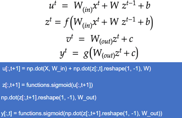
u[:,t+1] = np.dot(X, W_in) + np.dot(z[:,t].reshape(1, -1), W)
z[:,t+1] = functions.sigmoid(u[:,t+1])
y[:,t] = functions.sigmoid(np.dot(z[:,t+1].reshape(1, -1), W_out))
#誤差
loss = functions.mean_squared_error(dd, y[:,t])
delta_out[:,t] = functions.d_mean_squared_error(dd, y[:,t]) * functions.d_sigmoid(y[:,t])
all_loss += loss
out_bin[binary_dim - t - 1] = np.round(y[:,t])
for t in range(binary_dim)[::-1]:
X = np.array([a_bin[-t-1],b_bin[-t-1]]).reshape(1, -1)
delta[:,t] = (np.dot(delta[:,t+1].T, W.T) + np.dot(delta_out[:,t].T, W_out.T)) * functions.d_sigmoid(u[:,t+1])
# 勾配更新
W_out_grad += np.dot(z[:,t+1].reshape(-1,1), delta_out[:,t].reshape(-1,1))
W_grad += np.dot(z[:,t].reshape(-1,1), delta[:,t].reshape(1,-1))
W_in_grad += np.dot(X.T, delta[:,t].reshape(1,-1))
# 勾配適用
W_in -= learning_rate * W_in_grad
W_out -= learning_rate * W_out_grad
W -= learning_rate * W_grad
W_in_grad *= 0
W_out_grad *= 0
W_grad *= 0
if(i % plot_interval == 0):
all_losses.append(all_loss)
print("iters:" + str(i))
print("Loss:" + str(all_loss))
print("Pred:" + str(out_bin))
print("True:" + str(d_bin))
out_int = 0
for index,x in enumerate(reversed(out_bin)):
out_int += x * pow(2, index)
print(str(a_int) + " + " + str(b_int) + " = " + str(out_int))
print("------------")
lists = range(0, iters_num, plot_interval)
plt.plot(lists, all_losses, label="loss")
plt.show()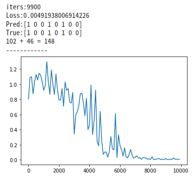
無事収束した。
import numpy as np
from common import functions
import matplotlib.pyplot as plt


def d_tanh(x):
   return 1/(np.cosh(x) ** 2)

# データを用意
# 2進数の桁数
binary_dim = 8
# 最大値 + 1
largest_number = pow(2, binary_dim)
# largest_numberまで2進数を用意
binary = np.unpackbits(np.array([range(largest_number)],dtype=np.uint8).T,axis=1)

input_layer_size = 2
hidden_layer_size = 16
output_layer_size = 1

weight_init_std = 1
learning_rate = 0.1

iters_num = 10000
plot_interval = 100

# ウェイト初期化 (バイアスは簡単のため省略)
W_in = weight_init_std * np.random.randn(input_layer_size, hidden_layer_size)
W_out = weight_init_std * np.random.randn(hidden_layer_size, output_layer_size)
W = weight_init_std * np.random.randn(hidden_layer_size, hidden_layer_size)
# Xavier
# W_in = np.random.randn(input_layer_size, hidden_layer_size) / (np.sqrt(input_layer_size))
# W_out = np.random.randn(hidden_layer_size, output_layer_size) / (np.sqrt(hidden_layer_size))
# W = np.random.randn(hidden_layer_size, hidden_layer_size) / (np.sqrt(hidden_layer_size))
# He
# W_in = np.random.randn(input_layer_size, hidden_layer_size) / (np.sqrt(input_layer_size)) * np.sqrt(2)
# W_out = np.random.randn(hidden_layer_size, output_layer_size) / (np.sqrt(hidden_layer_size)) * np.sqrt(2)
# W = np.random.randn(hidden_layer_size, hidden_layer_size) / (np.sqrt(hidden_layer_size)) * np.sqrt(2)


# 勾配
W_in_grad = np.zeros_like(W_in)
W_out_grad = np.zeros_like(W_out)
W_grad = np.zeros_like(W)

u = np.zeros((hidden_layer_size, binary_dim + 1))
z = np.zeros((hidden_layer_size, binary_dim + 1))
y = np.zeros((output_layer_size, binary_dim))

delta_out = np.zeros((output_layer_size, binary_dim))
delta = np.zeros((hidden_layer_size, binary_dim + 1))

all_losses = []

for i in range(iters_num):

   # A, B初期化 (a + b = d)
   a_int = np.random.randint(largest_number/2)
   a_bin = binary[a_int] # binary encoding
   b_int = np.random.randint(largest_number/2)
   b_bin = binary[b_int] # binary encoding

   # 正解データ
   d_int = a_int + b_int
   d_bin = binary[d_int]

   # 出力バイナリ
   out_bin = np.zeros_like(d_bin)

   # 時系列全体の誤差
   all_loss = 0

   # 時系列ループ
   for t in range(binary_dim):
       # 入力値
       X = np.array([a_bin[ - t - 1], b_bin[ - t - 1]]).reshape(1, -1)
       # 時刻tにおける正解データ
       dd = np.array([d_bin[binary_dim - t - 1]])

       u[:,t+1] = np.dot(X, W_in) + np.dot(z[:,t].reshape(1, -1), W)
       # z[:,t+1] = functions.sigmoid(u[:,t+1])
       z[:,t+1] = functions.relu(u[:,t+1])
#         z[:,t+1] = np.tanh(u[:,t+1])
       y[:,t] = functions.sigmoid(np.dot(z[:,t+1].reshape(1, -1), W_out))


       #誤差
       loss = functions.mean_squared_error(dd, y[:,t])

       delta_out[:,t] = functions.d_mean_squared_error(dd, y[:,t]) * functions.d_sigmoid(y[:,t])

       all_loss += loss

       out_bin[binary_dim - t - 1] = np.round(y[:,t])


   for t in range(binary_dim)[::-1]:
       X = np.array([a_bin[-t-1],b_bin[-t-1]]).reshape(1, -1)

       delta[:,t] = (np.dot(delta[:,t+1].T, W.T) + np.dot(delta_out[:,t].T, W_out.T)) * functions.d_sigmoid(u[:,t+1])
       # delta[:,t] = (np.dot(delta[:,t+1].T, W.T) + np.dot(delta_out[:,t].T, W_out.T)) * functions.d_relu(u[:,t+1])
       # delta[:,t] = (np.dot(delta[:,t+1].T, W.T) + np.dot(delta_out[:,t].T, W_out.T)) * d_tanh(u[:,t+1])

       # 勾配更新
       W_out_grad += np.dot(z[:,t+1].reshape(-1,1), delta_out[:,t].reshape(-1,1))
       W_grad += np.dot(z[:,t].reshape(-1,1), delta[:,t].reshape(1,-1))
       W_in_grad += np.dot(X.T, delta[:,t].reshape(1,-1))

   # 勾配適用
   W_in -= learning_rate * W_in_grad
   W_out -= learning_rate * W_out_grad
   W -= learning_rate * W_grad

   W_in_grad *= 0
   W_out_grad *= 0
   W_grad *= 0


   if(i % plot_interval == 0):
       all_losses.append(all_loss)
       print("iters:" + str(i))
       print("Loss:" + str(all_loss))
       print("Pred:" + str(out_bin))
       print("True:" + str(d_bin))
       out_int = 0
       for index,x in enumerate(reversed(out_bin)):
           out_int += x * pow(2, index)
       print(str(a_int) + " + " + str(b_int) + " = " + str(out_int))
       print("------------")

lists = range(0, iters_num, plot_interval)
plt.plot(lists, all_losses, label="loss")
plt.show()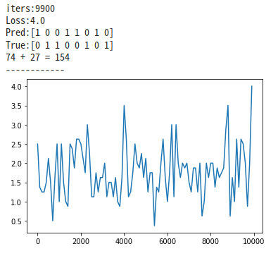
relu関数で処理した場合、収束できてなくlossが大きいことが分かる。
【確認テスト/考察結果】
確認テスト1:
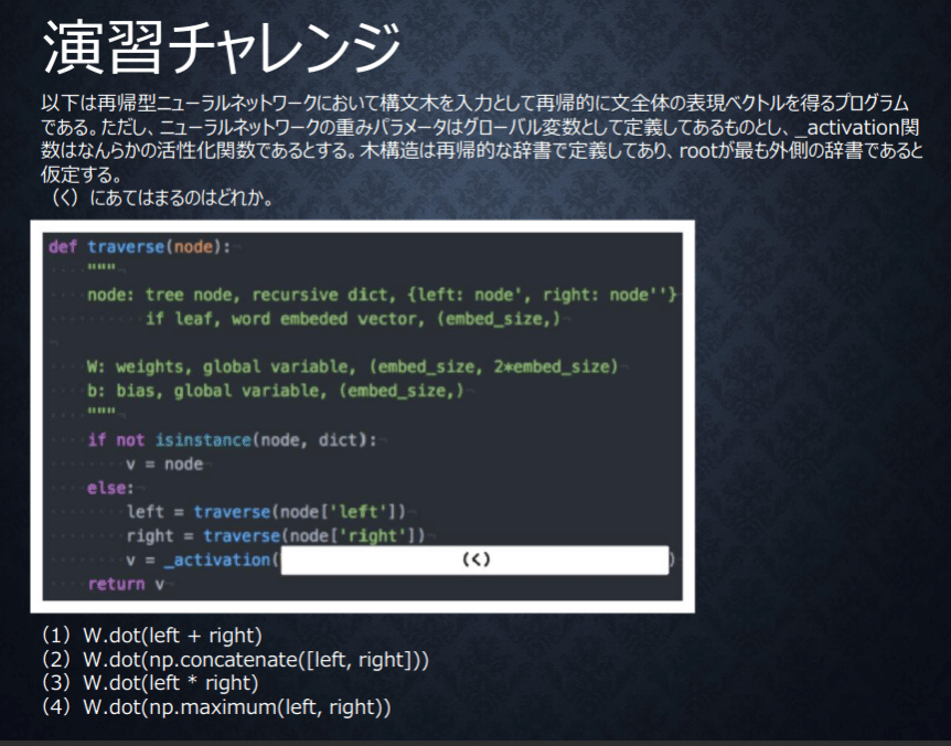
正直、再帰的な辞書で定義してある木構造がわかっていない。
今後学習で理解を深めるとして、今回は木構造の処理をどう考えるかに焦点を当てられている問題。left,rightをどう処理するのか。
考え方としてはleft,rightどちらも特徴を活かし再帰で展開していく、left,rightの足し算や引き算、大きい方を選ぶのであれば両方の特徴を活かせていない。
消去法で2番を選ぶことができる。
確認テスト2:
【関連/図書・問題・記事】
問題:
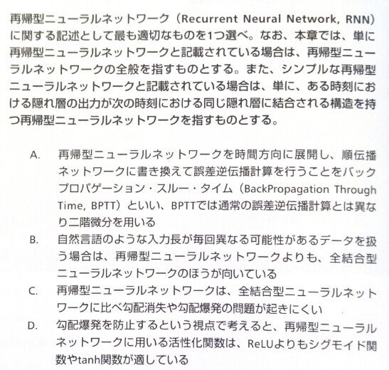
A、通常の誤差伝搬と同様に一階微分を用いるため不適切です
B、系列長の異なるデータを自然に扱えるのは再帰型ニューラルネットワークです。
C、再帰型ニューラルネットワークは全結合型ニューラルネットワークに比べて勾配消失や勾配爆発が起きやすい構造になっている。
答えはD
実装でのrelu関数を使用して勾配爆発が起こったことからもrelu関数を使用すると爆発が起きやすいことが分かる。
[ディープラーニングE資格問題集より]
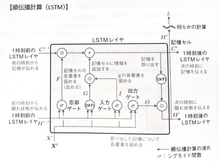
Section2:LSTM
【解説】
LSTM全体像:
RNN の課題
時系列を遡れば遡るほど、勾配が消失していく → 長い時系列の学習が困難
解決策
構造を変えることでその問題を解決したものを LSTM と言う。
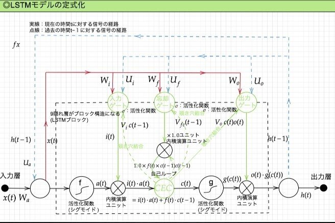
LSTM構造/2-1:CEC
問題と解決:
勾配消失および勾配爆発の問題があるが、解決方法として、勾配が 1 であれば解決できる。
課題と解決:
入力データについて、時間依存度に関係なく重みが一律であると言うことは、ニューラルネットワークの学習特性がそもそも失われてしまうという事。入力ゲートと出力ゲートを追加する事で解決する。
実際に入力と出力をどう使うのか解説する。
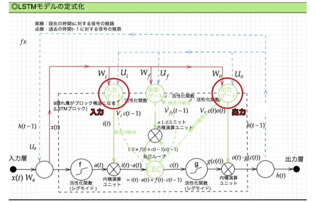
LSTM構造/2-2:入力ゲートと出力ゲート
入力ゲートと出力ゲートを追加することで
それぞれのゲートへの入力値の重みを重み行列 W,U で可変可能とする事でCEC の問題を解決する。
さらなる課題と解決策:
現状、すべての過去の情報をすべての情報が保管されるので過去の情報がいらなくなった場合削除できない。常に過去の情報に引っ張られているので、要らない過去の情報は削除する。解決策は忘却ゲート。
LSTM構造/2-3:忘却ゲート
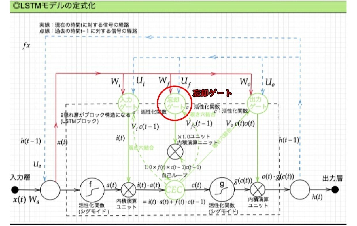
不要になった CEC の情報を削除するためのゲート
課題と解決策:
CEC の保存されている過去の情報を、任意のタイミングで他のノードに伝播させたり、あるいは任意のタイミングで忘却させたい。CEC 自身の値は、ゲート制御に影響を与えていない。のぞき穴結合にて影響を与えるようにする。
LSTM構造/2-3:除き穴結合
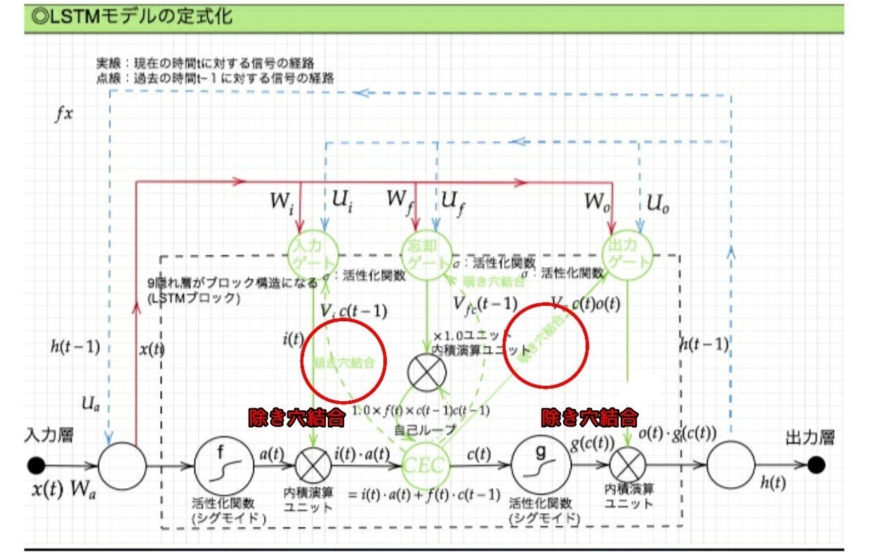
CEC自身の値に、重み行列を介して伝播可能にした構造。
【実装/演習】
LSTMをkerasにて実装:回帰
import pandas as pd
import numpy as np
import math
import random
import matplotlib.pyplot as plt
import seaborn as sns
# サイクルあたりのステップ数
steps_per_cycle = 80
# 生成するサイクル数
number_of_cycles = 50
df = pd.DataFrame(np.arange(steps_per_cycle * number_of_cycles + 1), columns=["t"])
# 一様乱数でノイズを発生させたsin波を生成
df["sin_t"] = df.t.apply(lambda x: math.sin(x * (2 * math.pi / steps_per_cycle)+ random.uniform(-0.05, +0.05) ))
# 2サイクルだけ抽出してプロット
df[["sin_t"]].head(steps_per_cycle * 2).plot()
# 画像を保存
plt.savefig('img_20190505085043.png')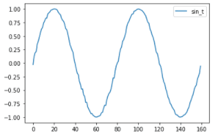
モデルの生成
(X_train, y_train), (X_test, y_test) = train_test_split(df[["sin_t"]])Kerasのバージョンの調整(バージョンが高い場合には動かない時がある)
pip install keras==2.3.1from keras.models import Sequential
from keras.layers.core import Dense, Activation
from keras.layers.recurrent import LSTM
# パラメータ
in_out_neurons = 1
hidden_neurons = 300
length_of_sequences = 30
model = Sequential()
model.add(LSTM(hidden_neurons, batch_input_shape=(None, length_of_sequences, in_out_neurons), return_sequences=False))
model.add(Dense(in_out_neurons))
model.add(Activation("linear"))
model.compile(loss="mean_squared_error", optimizer="rmsprop")
model.fit(X_train, y_train, batch_size=600, nb_epoch=15, validation_split=0.05)# 予測
predicted = model.predict(X_test)
# 描写
dataf = pd.DataFrame(predicted[:200])
dataf.columns = ["predict"]
dataf["input"] = y_test[:200]
dataf.plot()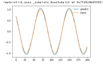
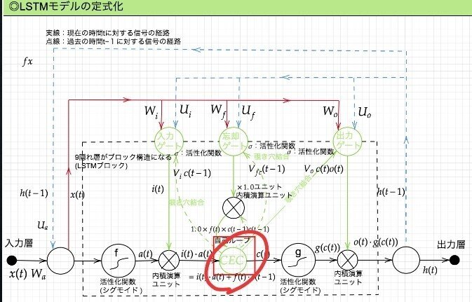
【確認テスト/考察結果】
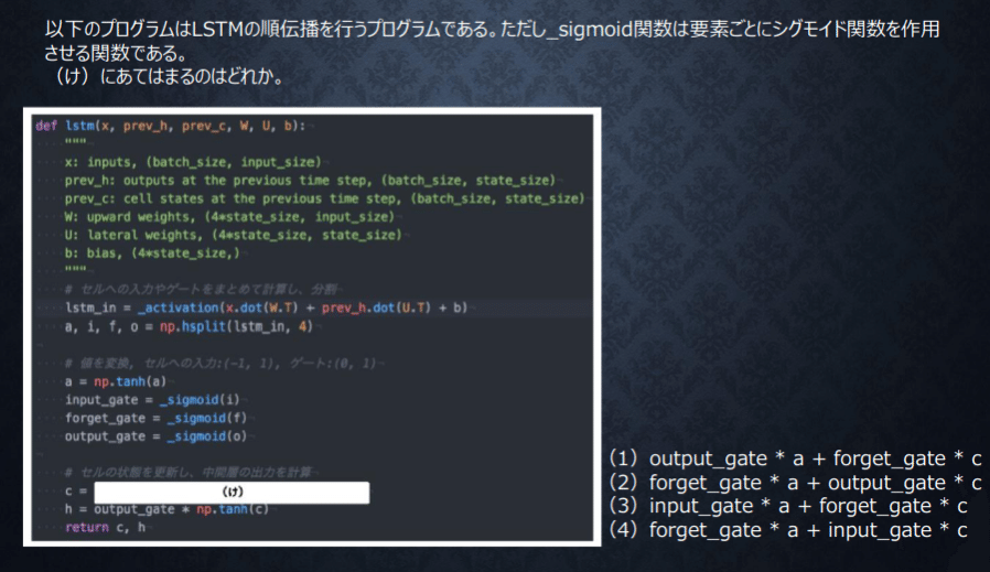
最後のhを見るとoutput_gete * np.tann(c)と書いてある
変数でなんでも名前をつけれるが、基本的にはすべて名前はちゃんとつけられていると考えていい様子。
もう少しみると、cは当然外から入ってきていない。aは外から?入ってきている。外から入ってきている変数はinput_gateと計算され、cは消去法でforget_getと計算されると考える。
あと、CはCECでCが形成されているのはどんな形かとのこと。するとoutput_geteは入ることはない。
【関連/図書・問題・記事】
問題:
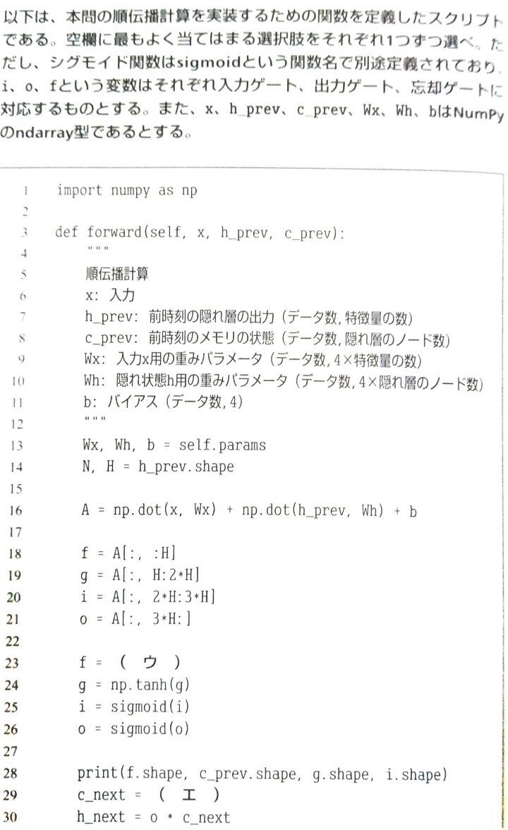
今回は参考に別の図を参考に考えてみる。
ウ = シグモイド関数にて、
sigmoid(f)エ = ネクストCなのでそれに該当しそうな部分はC+の右上の部分の出ていくC。それを構成するものは
f* c_prev+g*i Section3:GRU
【解説】
LSTM では、パラメータが多く計算負荷が高くなる問題があったので、GRUという手法が考えられた。
GRUは計算負荷が低い。
パラメータを大幅に削減し、精度は同等またはそれ以上が望める様になった。
GRU全体像:
【実装/演習】
%tensorflow_version 1.x
import logging
logging.getLogger("tensorflow").setLevel(logging.ERROR)
import tensorflow as tf
import numpy as np
import re
import glob
import collections
import random
import pickle
import time
import datetime
import os
# logging levelを変更
# tf.logging.set_verbosity(tf.logging.ERROR)
class Corpus:
def __init__(self):
self.unknown_word_symbol = "<???>" # 出現回数の少ない単語は未知語として定義しておく
self.unknown_word_threshold = 3 # 未知語と定義する単語の出現回数の閾値
self.corpus_file = "./corpus/**/*.txt"
self.corpus_encoding = "utf-8"
self.dictionary_filename = "./data_for_predict/word_dict.dic"
# self.dictionary_filename = "/content/drive/My Drive/DNN_code_colab_lesson_3_4/lesson_3/3_2_tf_languagemodel/data_for_predict/word_dict.dic"
# self.dictionary_filename = "drive/My Drive/DNN_code_colab_lesson_3_4/lesson_3/3_2_tf_languagemodel/data_for_predict/word_dict.dic"
self.chunk_size = 5
self.load_dict()
words = []
for filename in glob.glob(self.corpus_file, recursive=True):
with open(filename, "r", encoding=self.corpus_encoding) as f:
# word breaking
text = f.read()
# 全ての文字を小文字に統一し、改行をスペースに変換
text = text.lower().replace("\n", " ")
# 特定の文字以外の文字を空文字に置換する
text = re.sub(r"[^a-z '\-]", "", text)
# 複数のスペースはスペース一文字に変換
text = re.sub(r"[ ]+", " ", text)
# 前処理: '-' で始まる単語は無視する
words = [ word for word in text.split() if not word.startswith("-")]
self.data_n = len(words) - self.chunk_size
self.data = self.seq_to_matrix(words)
def prepare_data(self):
"""
訓練データとテストデータを準備する。
data_n = ( text データの総単語数 ) - chunk_size
input: (data_n, chunk_size, vocabulary_size)
output: (data_n, vocabulary_size)
"""
# 入力と出力の次元テンソルを準備
all_input = np.zeros([self.chunk_size, self.vocabulary_size, self.data_n])
all_output = np.zeros([self.vocabulary_size, self.data_n])
# 準備したテンソルに、コーパスの one-hot 表現(self.data) のデータを埋めていく
# i 番目から ( i + chunk_size - 1 ) 番目までの単語が1組の入力となる
# このときの出力は ( i + chunk_size ) 番目の単語
for i in range(self.data_n):
all_output[:, i] = self.data[:, i + self.chunk_size] # (i + chunk_size) 番目の単語の one-hot ベクトル
for j in range(self.chunk_size):
all_input[j, :, i] = self.data[:, i + self.chunk_size - j - 1]
# 後に使うデータ形式に合わせるために転置を取る
all_input = all_input.transpose([2, 0, 1])
all_output = all_output.transpose()
# 訓練データ:テストデータを 4 : 1 に分割する
training_num = ( self.data_n * 4 ) // 5
return all_input[:training_num], all_output[:training_num], all_input[training_num:], all_output[training_num:]
def build_dict(self):
# コーパス全体を見て、単語の出現回数をカウントする
counter = collections.Counter()
for filename in glob.glob(self.corpus_file, recursive=True):
with open(filename, "r", encoding=self.corpus_encoding) as f:
# word breaking
text = f.read()
# 全ての文字を小文字に統一し、改行をスペースに変換
text = text.lower().replace("\n", " ")
# 特定の文字以外の文字を空文字に置換する
text = re.sub(r"[^a-z '\-]", "", text)
# 複数のスペースはスペース一文字に変換
text = re.sub(r"[ ]+", " ", text)
# 前処理: '-' で始まる単語は無視する
words = [word for word in text.split() if not word.startswith("-")]
counter.update(words)
# 出現頻度の低い単語を一つの記号にまとめる
word_id = 0
dictionary = {}
for word, count in counter.items():
if count <= self.unknown_word_threshold:
continue
dictionary[word] = word_id
word_id += 1
dictionary[self.unknown_word_symbol] = word_id
print("総単語数:", len(dictionary))
# 辞書を pickle を使って保存しておく
with open(self.dictionary_filename, "wb") as f:
pickle.dump(dictionary, f)
print("Dictionary is saved to", self.dictionary_filename)
self.dictionary = dictionary
print(self.dictionary)
def load_dict(self):
with open(self.dictionary_filename, "rb") as f:
self.dictionary = pickle.load(f)
self.vocabulary_size = len(self.dictionary)
self.input_layer_size = len(self.dictionary)
self.output_layer_size = len(self.dictionary)
print("総単語数: ", self.input_layer_size)
def get_word_id(self, word):
# print(word)
# print(self.dictionary)
# print(self.unknown_word_symbol)
# print(self.dictionary[self.unknown_word_symbol])
# print(self.dictionary.get(word, self.dictionary[self.unknown_word_symbol]))
return self.dictionary.get(word, self.dictionary[self.unknown_word_symbol])
# 入力された単語を one-hot ベクトルにする
def to_one_hot(self, word):
index = self.get_word_id(word)
data = np.zeros(self.vocabulary_size)
data[index] = 1
return data
def seq_to_matrix(self, seq):
print(seq)
data = np.array([self.to_one_hot(word) for word in seq]) # (data_n, vocabulary_size)
return data.transpose() # (vocabulary_size, data_n)
class Language:
"""
input layer: self.vocabulary_size
hidden layer: rnn_size = 30
output layer: self.vocabulary_size
"""
def __init__(self):
self.corpus = Corpus()
self.dictionary = self.corpus.dictionary
self.vocabulary_size = len(self.dictionary) # 単語数
self.input_layer_size = self.vocabulary_size # 入力層の数
self.hidden_layer_size = 30 # 隠れ層の RNN ユニットの数
self.output_layer_size = self.vocabulary_size # 出力層の数
self.batch_size = 128 # バッチサイズ
self.chunk_size = 5 # 展開するシーケンスの数。c_0, c_1, ..., c_(chunk_size - 1) を入力し、c_(chunk_size) 番目の単語の確率が出力される。
self.learning_rate = 0.005 # 学習率
self.epochs = 1000 # 学習するエポック数
self.forget_bias = 1.0 # LSTM における忘却ゲートのバイアス
# self.model_filename = "drive/My Drive/DNN_code_colab_lesson_3_4/lesson_3/3_2_tf_languagemodel/data_for_predict/predict_model.ckpt"
# self.model_filename = "/content/drive/My Drive/DNN_code_colab_lesson_3_4/lesson_3/3_2_tf_languagemodel/data_for_predict/predict_model.ckpt"
self.model_filename = "./data_for_predict/predict_model.ckpt"
self.unknown_word_symbol = self.corpus.unknown_word_symbol
def inference(self, input_data, initial_state):
"""
:param input_data: (batch_size, chunk_size, vocabulary_size) 次元のテンソル
:param initial_state: (batch_size, hidden_layer_size) 次元の行列
:return:
"""
# 重みとバイアスの初期化
hidden_w = tf.Variable(tf.truncated_normal([self.input_layer_size, self.hidden_layer_size], stddev=0.01))
hidden_b = tf.Variable(tf.ones([self.hidden_layer_size]))
output_w = tf.Variable(tf.truncated_normal([self.hidden_layer_size, self.output_layer_size], stddev=0.01))
output_b = tf.Variable(tf.ones([self.output_layer_size]))
# BasicLSTMCell, BasicRNNCell は (batch_size, hidden_layer_size) が chunk_size 数ぶんつながったリストを入力とする。
# 現時点での入力データは (batch_size, chunk_size, input_layer_size) という3次元のテンソルなので
# tf.transpose や tf.reshape などを駆使してテンソルのサイズを調整する。
input_data = tf.transpose(input_data, [1, 0, 2]) # 転置。(chunk_size, batch_size, vocabulary_size)
input_data = tf.reshape(input_data, [-1, self.input_layer_size]) # 変形。(chunk_size * batch_size, input_layer_size)
input_data = tf.matmul(input_data, hidden_w) + hidden_b # 重みWとバイアスBを適用。 (chunk_size, batch_size, hidden_layer_size)
input_data = tf.split(input_data, self.chunk_size, 0) # リストに分割。chunk_size * (batch_size, hidden_layer_size)
# RNN のセルを定義する。RNN Cell の他に LSTM のセルや GRU のセルなどが利用できる。
cell = tf.nn.rnn_cell.BasicRNNCell(self.hidden_layer_size)
outputs, states = tf.nn.static_rnn(cell, input_data, initial_state=initial_state)
# 最後に隠れ層から出力層につながる重みとバイアスを処理する
# 最終的に softmax 関数で処理し、確率として解釈される。
# softmax 関数はこの関数の外で定義する。
output = tf.matmul(outputs[-1], output_w) + output_b
return output
def loss(self, logits, labels):
cost = tf.reduce_mean(tf.nn.softmax_cross_entropy_with_logits(logits=logits, labels=labels))
return cost
def training(self, cost):
# 今回は最適化手法として Adam を選択する。
# ここの AdamOptimizer の部分を変えることで、Adagrad, Adadelta などの他の最適化手法を選択することができる
optimizer = tf.train.AdamOptimizer(learning_rate=self.learning_rate).minimize(cost)
return optimizer
def train(self):
# 変数などの用意
input_data = tf.placeholder("float", [None, self.chunk_size, self.input_layer_size])
actual_labels = tf.placeholder("float", [None, self.output_layer_size])
initial_state = tf.placeholder("float", [None, self.hidden_layer_size])
prediction = self.inference(input_data, initial_state)
cost = self.loss(prediction, actual_labels)
optimizer = self.training(cost)
correct = tf.equal(tf.argmax(prediction, 1), tf.argmax(actual_labels, 1))
accuracy = tf.reduce_mean(tf.cast(correct, tf.float32))
# TensorBoard で可視化するため、クロスエントロピーをサマリーに追加
tf.summary.scalar("Cross entropy: ", cost)
summary = tf.summary.merge_all()
# 訓練・テストデータの用意
# corpus = Corpus()
trX, trY, teX, teY = self.corpus.prepare_data()
training_num = trX.shape[0]
# ログを保存するためのディレクトリ
timestamp = time.time()
dirname = datetime.datetime.fromtimestamp(timestamp).strftime("%Y%m%d%H%M%S")
# ここから実際に学習を走らせる
with tf.Session() as sess:
sess.run(tf.global_variables_initializer())
summary_writer = tf.summary.FileWriter("./log/" + dirname, sess.graph)
# エポックを回す
for epoch in range(self.epochs):
step = 0
epoch_loss = 0
epoch_acc = 0
# 訓練データをバッチサイズごとに分けて学習させる (= optimizer を走らせる)
# エポックごとの損失関数の合計値や(訓練データに対する)精度も計算しておく
while (step + 1) * self.batch_size < training_num:
start_idx = step * self.batch_size
end_idx = (step + 1) * self.batch_size
batch_xs = trX[start_idx:end_idx, :, :]
batch_ys = trY[start_idx:end_idx, :]
_, c, a = sess.run([optimizer, cost, accuracy],
feed_dict={input_data: batch_xs,
actual_labels: batch_ys,
initial_state: np.zeros([self.batch_size, self.hidden_layer_size])
}
)
epoch_loss += c
epoch_acc += a
step += 1
# コンソールに損失関数の値や精度を出力しておく
print("Epoch", epoch, "completed ouf of", self.epochs, "-- loss:", epoch_loss, " -- accuracy:",
epoch_acc / step)
# Epochが終わるごとにTensorBoard用に値を保存
summary_str = sess.run(summary, feed_dict={input_data: trX,
actual_labels: trY,
initial_state: np.zeros(
[trX.shape[0],
self.hidden_layer_size]
)
}
)
summary_writer.add_summary(summary_str, epoch)
summary_writer.flush()
# 学習したモデルも保存しておく
saver = tf.train.Saver()
saver.save(sess, self.model_filename)
# 最後にテストデータでの精度を計算して表示する
a = sess.run(accuracy, feed_dict={input_data: teX, actual_labels: teY,
initial_state: np.zeros([teX.shape[0], self.hidden_layer_size])})
print("Accuracy on test:", a)
def predict(self, seq):
"""
文章を入力したときに次に来る単語を予測する
:param seq: 予測したい単語の直前の文字列。chunk_size 以上の単語数が必要。
:return:
"""
# 最初に復元したい変数をすべて定義してしまいます
# tf.reset_default_graph()
tf.compat.v1.reset_default_graph()
input_data = tf.placeholder("float", [None, self.chunk_size, self.input_layer_size])
initial_state = tf.placeholder("float", [None, self.hidden_layer_size])
prediction = tf.nn.softmax(self.inference(input_data, initial_state))
predicted_labels = tf.argmax(prediction, 1)
# 入力データの作成
# seq を one-hot 表現に変換する。
words = [word for word in seq.split() if not word.startswith("-")]
x = np.zeros([1, self.chunk_size, self.input_layer_size])
for i in range(self.chunk_size):
word = seq[len(words) - self.chunk_size + i]
index = self.dictionary.get(word, self.dictionary[self.unknown_word_symbol])
x[0][i][index] = 1
feed_dict = {
input_data: x, # (1, chunk_size, vocabulary_size)
initial_state: np.zeros([1, self.hidden_layer_size])
}
# tf.Session()を用意
with tf.Session() as sess:
# 保存したモデルをロードする。ロード前にすべての変数を用意しておく必要がある。
saver = tf.train.Saver()
saver.restore(sess, self.model_filename)
# ロードしたモデルを使って予測結果を計算
u, v = sess.run([prediction, predicted_labels], feed_dict=feed_dict)
keys = list(self.dictionary.keys())
# コンソールに文字ごとの確率を表示
for i in range(self.vocabulary_size):
c = self.unknown_word_symbol if i == (self.vocabulary_size - 1) else keys[i]
print(c, ":", u[0][i])
print("Prediction:", seq + " " + ("<???>" if v[0] == (self.vocabulary_size - 1) else keys[v[0]]))
return u[0]
def build_dict():
cp = Corpus()
cp.build_dict()
if __name__ == "__main__":
#build_dict()
ln = Language()
# 学習するときに呼び出す
#ln.train()
# 保存したモデルを使って単語の予測をする
ln.predict("some of them looks like")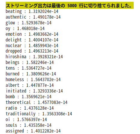
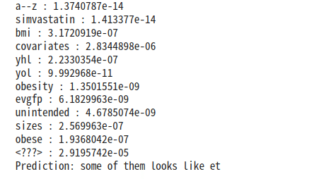
文字が約9800くらいだったので、5000で切り捨てられてる。数えると、きっちり5000表示されているので、出現回数の多い単語から表示されて、5000以降は<???>に分類されていると思われる。
>>self.unknown_word_symbol = "<???>" # 出現回数の少ない単語は未知語として定義しておく<<
TOP5000以下の出現回数の少ない<???>がなんだかんだ一番多い。
【確認テスト/考察結果】

LSTM:4つの部品を持つことで構成され、非常に計算量が多くなることが課題。
CEC:学習が出来ないことが課題。そのためゲートをつけて学習をしている。
つまり、CECが学習できないため部品が多くなり、計算量が非常に多くなっているということ。
【関連/図書・問題・記事】
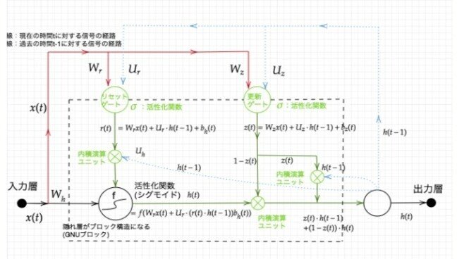
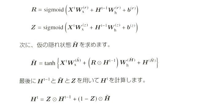
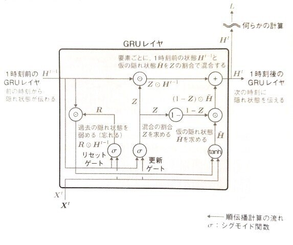
GRU順伝搬の計算:
GRUレイヤへの入力はxtと、1時刻前の出力であるhT-1でありHtが出力されているLSTMと違い記憶セルはありません。パラメータとしては重み行列であるWとBがある。

まずリセットゲートの値Rと更新ゲートのZを計算。
GRU順伝搬参考図:
[ディープラーニングE資格問題集より]
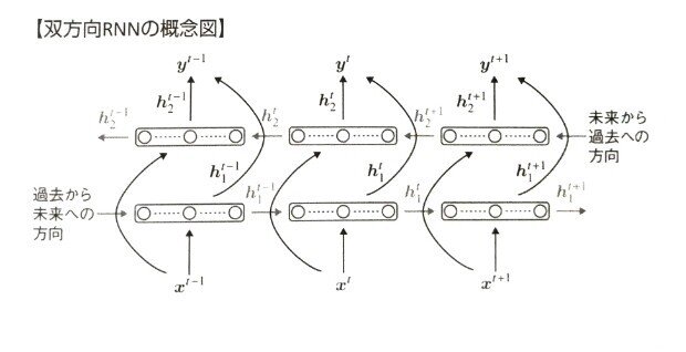
Section4:双方向RNN
【解説】
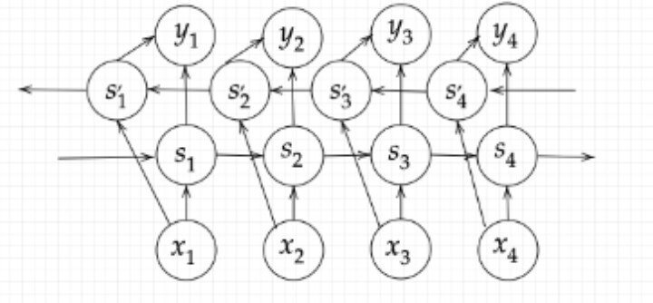
双方向RNN過去の情報だけでなく、未来の情報を加味することで、精度を向上させるためのモデるで、文章の推敲や、機械翻訳等に利用される。
【確認テスト/考察結果】
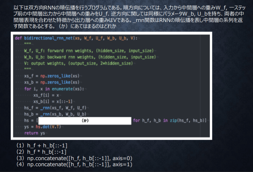
特徴を活かしつつ次のステップに行くにはそれぞれ特徴を記録する。行列として記録しないと、それぞれがわからないのでその記録ができるのは4番となる。
【関連/図書・問題・記事】
過去から未来、未来から過去へ方向も考慮した再帰型ニューラルネットワーク例えば文章内の文字の穴埋めタスクなど過去から現在から未来まで情報を用いることで有効と考えられている手法。
[ディープラーニングE資格問題集より]
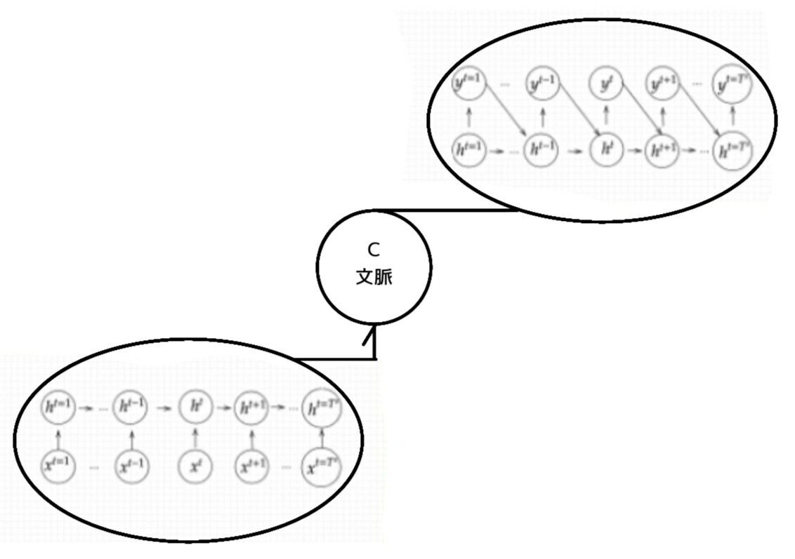
Section5:Seq2Seq
【解説】
Seq2seqは機械対話や、機械翻訳などに使用されている。
全体像:
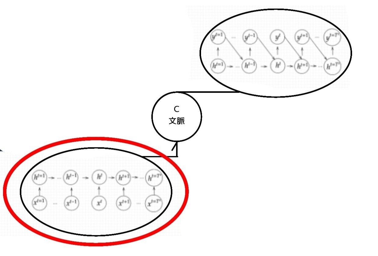
Seq2Seq構造/5-1:Encoder RNN
ユーザーがインプットしたテキストデータを、単語等のトークンに区切って渡す構造。
文章を単語等のトークン毎に分割し、トークンごとのIDに分割する。Embedding :IDから、そのトークンを表す分散表現ベクトルに変換。Encoder RNN:ベクトルを順番にRNNに入力していく。
処理手順:
vec1をRNNに入力し、hidden stateを出力。このhiddenstateと次の入力vec2をまたRNNに入力してきたhidden stateを出力という流れを繰り返す。・最後のvecを入れたときのhiddenstateをfinalstateとしてとっておく。このfinalstateがthoughtvectorと呼ばれ、入力した文の意味を表すベクトルとなる。
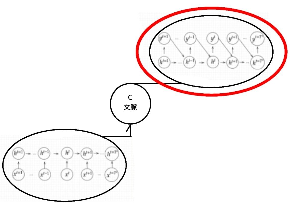
Seq2Seq構造/5-2:Decoder RNN
システムがアウトプットデータを、単語等のトークンごとに生成する構造。
処理手順:
1.Decoder RNN: Encoder RNN のfinal state (thought vector) から、各token の生成確率を出力していきますfinal state をDecoder RNN のinitial state ととして設定し、Embedding を入力。
2.Sampling:生成確率にもとづいてtoken をランダムに選びます。3.Embedding:2で選ばれたtoken をEmbedding してDecoder RNN への次の入力とします。4.Detokenize:1 -3 を繰り返し、2で得られたtoken を文字列に直します。
課題と解決:
一問一答しかできない問に対して文脈も何もなく、ただ応答が行われる続ける。その結果、改善としてHREDが考え出された。
5-3:HRED
Seq2Seq + Context RNNの構造です。
過去の発話から次の発話を生成。
HREDでは、前の単語の流れに即して応答されるため、より人間らしい文章が生成される。
課題
会話の流れのような多様性がなく、同じ発話に対して同じような発話がされる
短く情報量に乏しい発話(うん、そうだね、…etc)をしがち
5-3:VEA
オートエンコーダ(Auto Encoder)
オートエンコーダとは、教師なし学習。
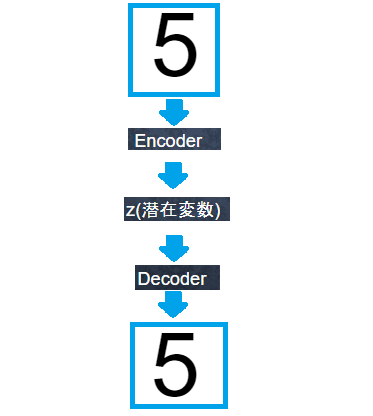
Encoder:入力データから潜在変数zに変換するニューラルネットワーク
Decoder:潜在変数zから元画像を復元するニューラルネットワーク
出力した画像の潜在変数zが入力画像より小さくなっていれば次元削減とみなす。その他、ノイズ除去や異常検知に使用される。
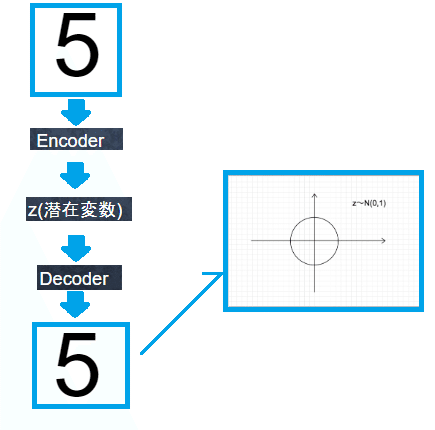
VAE(Variational Autoencoder)
通常のオートエンコーダーの場合、何かしら潜在変数zにデータを押し込めているものの、その構造がどのような状態不明。
VAEはこの潜在変数zに確率分布z〜N(0,1)を仮定したもの。
【確認テスト/考察結果】
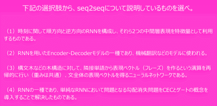
<解答>
(2)
(1)は双方向RNNについての説明(3)は構文木についての説明(4)はLSTMについての説明となっている様子。
【関連/図書・問題・記事】
機械学習界隈ではブレイクスルーな技術としてGANやVAEが話題となった。今回解説するSeq2Seqもブレイクスルーといわれる技術の1つ。
近年、劇的に日本語の翻訳技術が向上。その技術の背景にはSeq2Seqが使われている。Seq2Seqの得意分野は翻訳も、自動字幕技術、あるいはチャットボットなどのQuestions answeringの技術であり、連続値などのシーケンシャルなデータの取扱が得意。
Seq2SeqはGoogleにより2014年に発表。Googleは2015年頃の論文でSpeech recognitionやビデオ字幕で劇的に精度が向上したと発表している。
特徴:
Seq2Seqは2つのパートに別れ、EncoderとDecoder。形的にはAutoEncoder(例えばVAE)に少し似ているが、中の実装方式がまるで違う。
Seq2SeqはRNNを利用しているため時系列データに強いという所が特徴。 そのため翻訳や音声認識の分野で力を発揮している。
[関連記事より]
Section6:Word2vec
【解説】
RNNでは、単語のような可変長の文字列をNNに与えることはできないため、固定長形式で単語を表す必要がある。
そこで、分布仮説から単語を固定長のベクトル化(単語分散表現ベクトル)するソフトウェアのWord2vecが考えられた。
学習データからボキャブラリーを作成し、
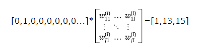
各単語をone-hotベクトルにして入力して単語分散表現,大規模データの分散表現の学習が、現実的な計算速度とメモリ量で実現可能になった。
ボキャブラリ × 任意の単語のベクトル表現(単語の変換表)を機械学習で学習することで、計算速度を向上した。
【確認テスト/考察結果】

RNN時系列データの処理に適しているネットワーク。word2vec単語の分散表現を得る手法。seq2seq一つの時系列データから別の時系列データを得る手法、Attentionそれぞれの時系列データに重みをつける手法。
【関連/図書・問題・記事】
[ディープラーニングE資格問題集より]
Section7:Attention Mechanism
【解説】
Seq2Seqは文章の単語数に関わらず常に固定次元ベクトルで入力しなければならないため、長い文章への対応が難しい。
(Seq2Seqでは2単語でも、100単語でも、固定次元ベクトルの中に入力しなければならない。)
対応策:
この問題の解決策として、文章が長くなるほどそのシーケンスの内部表現の次元も大きくなっていく仕組みが必要。関連度を学習することで関連度が高い部分を抽出して効率的に処理を行なう。
【確認テスト/考察結果】

seq2seqは会話の文脈を無視した処理を行うといった課題があったが、HREDは文脈の流れを考慮した処理を行う
HREDは短く情報量の乏しいな返事しかできない課題があったが、VHREDはHREDの課題をVAEの潜在変数の概念を追加して解決したもの。
【関連/図書・問題・記事】
通常のエンコーダ・デコーダモデルでは、エンコーダの出力は一つの様子。使い方はそれぞれ。この方法では、入力文の情報を特定のサイズのベクトルにまとめる必要があり、長文になればなるほど元の情報の圧縮精度が悪くなる。
一方、attention を用いたモデルでは、エンコーダーの隠れ層のうち、特定の入力単語やその周辺の単語にフォーカスしたベクトルをデコーダで使えるので、デコーダのある時点で必要な情報にフォーカスして使用することができ、入力文の長さに関係なくデコードを効率よく行える。
attention の使い方もいろいろ有るが、すべてのベクトルを重み付けして利用する global attention や特定のベクトルのみを用いる local attention と呼ばれる方法に分けている提案も有る様子。
[最近のDeep Learning (NLP) 界隈におけるAttention事情 ]
からの分かる部分だけ見た大きな概要
この記事が気に入ったらサポートをしてみませんか?