2024年2月に発表された時系列予測のためのLag-Llamaモデル

Lag-Llamaとは?
Lag-Llamaは最近発表された時系列予測のためのオープンソースモデルです。
様々なドメインにわたる広範囲の時系列データでトレーニングされています。
公式のGithubレポジトリにあるデモを参考にLag-Llamaでゼロショット予測を試してみます。環境はGoogle Corabです。
インストール
Lag-LlamaのGithubレポジトリから取得してインストールを行います。
!git clone https://github.com/time-series-foundation-models/lag-llama/
cd /content/lag-llama
!pip install -r requirements.txt --quiet
事前学習済みのモデルのウェイトを取得
HuggingFaceから事前学習済みのモデルのウェイトをダウンロードしています。
!huggingface-cli download time-series-foundation-models/Lag-Llama lag-llama.ckpt --local-dir /content/lag-llamaライブラリの読み込み
from itertools import islice

from matplotlib import pyplot as plt
import matplotlib.dates as mdates

import torch
from gluonts.evaluation import make_evaluation_predictions, Evaluator
from gluonts.dataset.repository.datasets import get_dataset

from gluonts.dataset.pandas import PandasDataset
import pandas as pd

from lag_llama.gluon.estimator import LagLlamaEstimator
Lag-Llamaで予測を行うための関数
def get_lag_llama_predictions(dataset, prediction_length, num_samples=100):
    ckpt = torch.load("lag-llama.ckpt", map_location=torch.device('cuda:0')) # GPUを利用しています。
    estimator_args = ckpt["hyper_parameters"]["model_kwargs"]

    estimator = LagLlamaEstimator(
        ckpt_path="lag-llama.ckpt",
        prediction_length=prediction_length,
        context_length=32, # 事前学習済みのモデルが訓練された設定であるため、変更してはいけない。

        # estimator args
        input_size=estimator_args["input_size"],
        n_layer=estimator_args["n_layer"],
        n_embd_per_head=estimator_args["n_embd_per_head"],
        n_head=estimator_args["n_head"],
        scaling=estimator_args["scaling"],
        time_feat=estimator_args["time_feat"],

        batch_size=1,
        num_parallel_samples=100
    )

    lightning_module = estimator.create_lightning_module()
    transformation = estimator.create_transformation()
    predictor = estimator.create_predictor(transformation, lightning_module)

    forecast_it, ts_it = make_evaluation_predictions(
        dataset=dataset,
        predictor=predictor,
        num_samples=num_samples
    )
    forecasts = list(forecast_it)
    tss = list(ts_it)

    return forecasts, tss
予測を行うための関数を見てみます。大まかに以下の処理を行なっています。
取得した事前学習済みのモデルをロード
ハイパーパラメーターを取得
LagLlamaEstimatorで推定器を作成
予測器を作成(create_predictor)
予測(make_evaluation_predictions)
最終的に予測された時系列データを返します
1で先ほど取得した事前学習済みのモデルのウェイトのチェックポイントファイルであるlag-llama.ckptをロードしています。cuda:0を指定しているため、GPU環境を想定しています。Google Corabの場合は、ランタイムのタイプを変更することでGPU環境に変更できます。
データセットの読み込み
import pandas as pd
from gluonts.dataset.pandas import PandasDataset

url = (
    "https://gist.githubusercontent.com/rsnirwan/a8b424085c9f44ef2598da74ce43e7a3"
    "/raw/b6fdef21fe1f654787fa0493846c546b7f9c4df2/ts_long.csv"
)
df = pd.read_csv(url, index_col=0, parse_dates=True)
df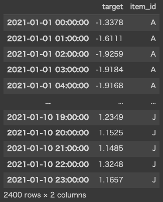
for col in df.columns:
    if df[col].dtype != 'object' and pd.api.types.is_string_dtype(df[col]) == False:
        df[col] = df[col].astype('float32')

dataset = PandasDataset.from_long_dataframe(df, target="target", item_id="item_id")

backtest_dataset = dataset
prediction_length = 24  # 予測期間を定義します。ここではデータが1時間毎の頻度であるため、24を使用します。
num_samples = 100 # 確率分布からサンプリングされるサンプルの数です。
予測を行う
先ほど定義した関数で予測を行います。
forecasts, tss = get_lag_llama_predictions(backtest_dataset, prediction_length, num_samples)予測の可視化
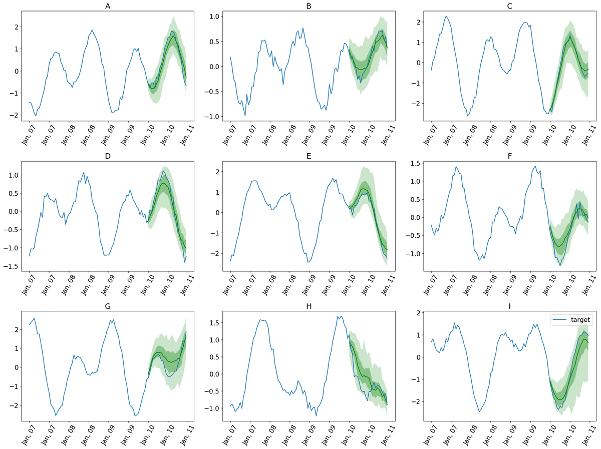
plt.figure(figsize=(20, 15))
date_formater = mdates.DateFormatter('%b, %d')
plt.rcParams.update({'font.size': 15})

for idx, (forecast, ts) in islice(enumerate(zip(forecasts, tss)), 9):
    ax = plt.subplot(3, 3, idx+1)

    plt.plot(ts[-4 * prediction_length:].to_timestamp(), label="target", )
    forecast.plot( color='g')
    plt.xticks(rotation=60)
    ax.xaxis.set_major_formatter(date_formater)
    ax.set_title(forecast.item_id)

plt.gcf().tight_layout()
plt.legend()
plt.show()