Keras 3でテーブルデータのディープラーニング

Kerasとは?
Kerasはディープラーニングのフレームワークです。昨年の11月にバージョン3.0.0がリリースされ、バックエンドとしてJAX, PyTorch, TensorFlowを利用することが出来るようになりました。シンプルなAPIを提供してるため、直感的にディープラーニングのモデルを扱う事ができるようになっています。
この記事では最新バージョンのKeras 3でテーブルデータに対するディープラーニングを行ってみたいと思います。ドキュメンテーションにあるサンプルを参考にGoogle Corabで動かしてみたいと思います。
インストール
pip install --upgrade kerasKerasをインストールします。
import keras
print(keras.__version__)
3.1.1
バージョンを確認しておきます。最新版の3.1.1がインストールされていることが確認できます。
import os

os.environ["KERAS_BACKEND"] = "tensorflow"
バックエンドにTensorFlowを指定しています。
ライブラリの読み込み
import tensorflow as tf
import pandas as pd
import keras
from keras import layers
データセットの読み込み
file_url = "http://storage.googleapis.com/download.tensorflow.org/data/heart.csv"
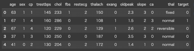
dataframe = pd.read_csv(file_url)データセットの読み込みを行います。
今回利用するデータセットはクリーブランドクリニック財団から提供されている心臓病に関するデータで全部で303行のCSVファイルです。各行には患者に関する特徴量が含まれています。これらの特徴量を使用して、患者が心臓病を持っているかどうかを予測する二値分類問題になります。
訓練用と検証用にデータを分割
val_dataframe = dataframe.sample(frac=0.2, random_state=1337)
train_dataframe = dataframe.drop(val_dataframe.index)

print(
    f"{len(train_dataframe)} サンプルを訓練用に使用します"
    f" {len(val_dataframe)} サンプルを検証用に使用します"
)
242 サンプルを訓練用に使用します 61 サンプルを検証用に使用します
訓練用と検証用にデータを分割しています。
def dataframe_to_dataset(dataframe):
    dataframe = dataframe.copy()
    labels = dataframe.pop("target")
    ds = tf.data.Dataset.from_tensor_slices((dict(dataframe), labels))
    ds = ds.shuffle(buffer_size=len(dataframe))
    return ds


train_ds = dataframe_to_dataset(train_dataframe)
val_ds = dataframe_to_dataset(val_dataframe)PandasのデータフレームをTensorFlowのデータセット(tf.data.Dataset)に変換する関数を定義しています。
この関数を訓練用と検証用のデータそれぞれに適用します。
train_ds = train_ds.batch(32)
val_ds = val_ds.batch(32)
データセットを32個のサンプルを含むバッチに分割しています。
特徴量エンジニアリング
特徴量エンジニアリングを行うための関数を定義しています。
encode_numerical_feature:数値の特徴量に対して正規化を適用する。
encode_categorical_feature:カテゴリの特徴量に対してOne-Hotエンコーディングを適用する。
def encode_numerical_feature(feature, name, dataset):
    normalizer = layers.Normalization()

    feature_ds = dataset.map(lambda x, y: x[name])
    feature_ds = feature_ds.map(lambda x: tf.expand_dims(x, -1))

    normalizer.adapt(feature_ds)

    encoded_feature = normalizer(feature)
    return encoded_feature


def encode_categorical_feature(feature, name, dataset, is_string):
    lookup_class = layers.StringLookup if is_string else layers.IntegerLookup
    lookup = lookup_class(output_mode="binary")

    feature_ds = dataset.map(lambda x, y: x[name])
    feature_ds = feature_ds.map(lambda x: tf.expand_dims(x, -1))

    lookup.adapt(feature_ds)

    encoded_feature = lookup(feature)
    return encoded_feature
モデルの構築
# 数値でエンコードされたカテゴリ特徴量
sex = keras.Input(shape=(1,), name="sex", dtype="int64")
cp = keras.Input(shape=(1,), name="cp", dtype="int64")
fbs = keras.Input(shape=(1,), name="fbs", dtype="int64")
restecg = keras.Input(shape=(1,), name="restecg", dtype="int64")
exang = keras.Input(shape=(1,), name="exang", dtype="int64")
ca = keras.Input(shape=(1,), name="ca", dtype="int64")

# 文字列でエンコードされたカテゴリ特徴量
thal = keras.Input(shape=(1,), name="thal", dtype="string")

# 数値の特徴量
age = keras.Input(shape=(1,), name="age")
trestbps = keras.Input(shape=(1,), name="trestbps")
chol = keras.Input(shape=(1,), name="chol")
thalach = keras.Input(shape=(1,), name="thalach")
oldpeak = keras.Input(shape=(1,), name="oldpeak")
slope = keras.Input(shape=(1,), name="slope")

all_inputs = [
    sex,
    cp,
    fbs,
    restecg,
    exang,
    ca,
    thal,
    age,
    trestbps,
    chol,
    thalach,
    oldpeak,
    slope,
]

# 数値のカテゴリ特徴量
sex_encoded = encode_categorical_feature(sex, "sex", train_ds, False)
cp_encoded = encode_categorical_feature(cp, "cp", train_ds, False)
fbs_encoded = encode_categorical_feature(fbs, "fbs", train_ds, False)
restecg_encoded = encode_categorical_feature(restecg, "restecg", train_ds, False)
exang_encoded = encode_categorical_feature(exang, "exang", train_ds, False)
ca_encoded = encode_categorical_feature(ca, "ca", train_ds, False)

# 文字列のカテゴリ特徴量
thal_encoded = encode_categorical_feature(thal, "thal", train_ds, True)

# 数値の特徴量
age_encoded = encode_numerical_feature(age, "age", train_ds)
trestbps_encoded = encode_numerical_feature(trestbps, "trestbps", train_ds)
chol_encoded = encode_numerical_feature(chol, "chol", train_ds)
thalach_encoded = encode_numerical_feature(thalach, "thalach", train_ds)
oldpeak_encoded = encode_numerical_feature(oldpeak, "oldpeak", train_ds)
slope_encoded = encode_numerical_feature(slope, "slope", train_ds)

all_features = layers.concatenate(
    [
        sex_encoded,
        cp_encoded,
        fbs_encoded,
        restecg_encoded,
        exang_encoded,
        slope_encoded,
        ca_encoded,
        thal_encoded,
        age_encoded,
        trestbps_encoded,
        chol_encoded,
        thalach_encoded,
        oldpeak_encoded,
    ]
)
x = layers.Dense(32, activation="relu")(all_features)
x = layers.Dropout(0.5)(x)
output = layers.Dense(1, activation="sigmoid")(x)
model = keras.Model(all_inputs, output)
model.compile("adam", "binary_crossentropy", metrics=["accuracy"])
特徴エンジニアリングを実施してモデルを構築します。
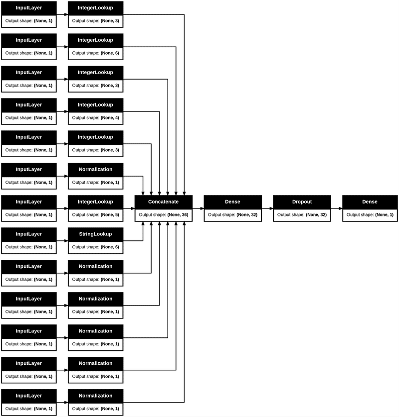
keras.utils.plot_model(model, show_shapes=True, rankdir="LR")構築したモデルのネットワークを可視化しています。
学習
fit()で学習を行います。
エポック数は50回と指定されています。
model.fit(train_ds, epochs=50, validation_data=val_ds)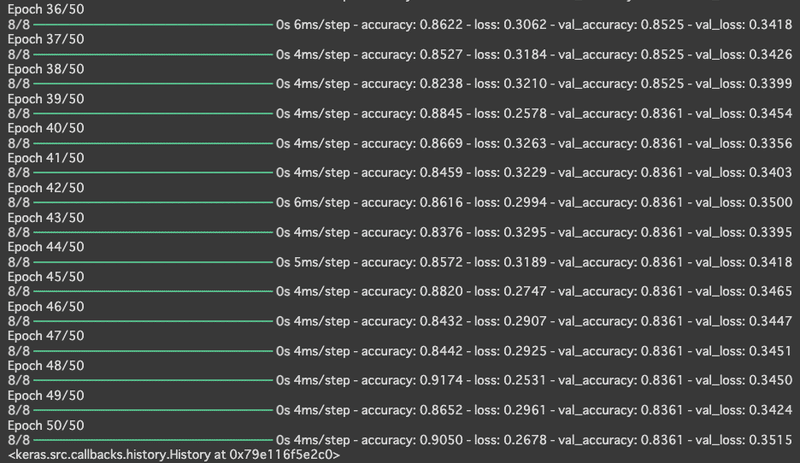
予測
予測については、predict()で行う事ができます。
sample = {
"age": 60,
"sex": 1,
"cp": 1,
"trestbps": 145,
"chol": 233,
"fbs": 1,
"restecg": 2,
"thalach": 150,
"exang": 0,
"oldpeak": 2.3,
"slope": 3,
"ca": 0,
"thal": "fixed",
}
input_dict = {name: tf.convert_to_tensor([value]) for name, value in sample.items()}
predictions = model.predict(input_dict)
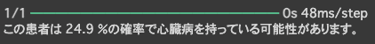
print(
f"この患者は {100 * predictions[0][0]:.1f} "
"%の確率で心臓病を持っている可能性があります。"
)