
2.モデル作成 : 実践的ボートレース(競艇)予想AIを作ろう

[注意]掲載しているコード等は執筆時点では動いていますが、その後の環境の変化等により動かなくなっていることがあります。コードが必ず動くことを保証する訳ではありません。あくまでも参考にしてください。
0.この記事ですること
データの取得には時間がかかるので、取得している間にモデル作成を進めたいと思います。
この記事では、モデル作成 ~ テストのまでの流れを簡単に解説し、1位かどうか?を予測するモデルを作ります。
※使っているTableなどは、前回の記事で作成しています。
▼ 「実践的ボートレース(競艇)予想AIを作ろう」 のnote全体は下記から
1.処理の流れ
まずはざっくりと処理の流れを説明します。
1.DBから「レース情報&直前情報 」と「結果」を取り出す
2.「レース情報&直前情報 」から使える特徴量をピックアップする
3.「結果」と結合する(1位だったかどうかを判別するため)
4.作ったリストを3分割する(モデル作成用/テスト用/シミュレーション用)
5.LightGBMを使って学習~モデル作成する
6.作ったモデルでシミュレーションする
2.コード解説
※今回はモデル作りのお試しなので、新しいcolabのファイルを用意してください。
1.設定
!pip install pandas
!pip install mysql-connector-python
!pip install LightGBM
!pip install japanize-matplotlib
!pip install optuna


import numpy as np
import lightgbm as lgb
import pandas as pd
import mysql.connector
from mysql.connector import errorcode
import sys
import warnings
import sqlalchemy
import pandas as pd
# import optuna.integration.lightgbm as lgb
import lightgbm as lgb
import numpy as np
from sklearn.metrics import mean_squared_error
import pickle
from google.colab import drive
import os
from PIL import Image
from sklearn import metrics
import datetime

warnings.filterwarnings('ignore')
2.Mysqlへの接続部分
class TableManager:
    def __init__(self, host, username, password, database):
        self.host = host
        self.username = username
        self.password = password
        self.database = database
        self.connection = None
        self.chunk_size = 1000
    def connect(self):
        try:
            self.connection = mysql.connector.connect(
                host=self.host,
                user=self.username,
                password=self.password,
                database=self.database,
                port=3306  # ポート番号がデフォルトの3306の場合
            )

            # 接続が成功したか確認
            if self.connection.is_connected():
                # print("\nMySQLに接続しました。")
                print("")

        except mysql.connector.Error as err:
            print(f"\nエラー: {err}")
    def disconnect(self):
        if self.connection and self.connection.is_connected():
            self.connection.close()
            # print("\nMySQL接続を閉じました.")
    def execute_query(self, query):
        cursor = self.connection.cursor(dictionary=True)
        try:
            cursor.execute(query)
            result = cursor.fetchall()
            return result
        except mysql.connector.Error as err:
            print(f"クエリの実行中にエラーが発生しました: {err}")
        finally:
            cursor.close()

manager = TableManager(
    host="xxxxxxxxxxx",
    username="xxxxxxxxxx",
    password="xxxxxxxxx",
    database="xxxxxxxxxx"
)
host="xxxxxxxxxxx",
username="xxxxxxxxxx",
password="xxxxxxxxx",
database="xxxxxxxxxx"
の部分は、自身の環境に合わせてください
3.データ取得
query_1 = '''
/* 出走前にわかっている情報 */
select
*
from schedule
inner join recent_weather using( race_date , jcd , race_no )
inner join entries using( race_date , jcd , race_no )
inner join rankingmotor using( race_date , jcd , racer_no )
inner join recent_start_exhibition using( race_date , jcd , race_no , waku )
where race_date between '2023-01-01' and '2023-12-31'
'''

query_2 = '''
/* 出走後にわかる情報&結果 */
select
*
from schedule
inner join result_weather using( race_date , jcd , race_no )
inner join result_racers using( race_date , jcd , race_no )
inner join result_start using( race_date , jcd , race_no , waku )
where race_date between '2023-01-01' and '2023-12-31'
'''

manager.connect()

# クエリを実行して結果を取得
results_recent = manager.execute_query(query_1)
results_result = manager.execute_query(query_2)

# 結果をDataFrameに変換
df_recent = pd.DataFrame(results_recent)
df_result = pd.DataFrame(results_result)
query_1 は、出走前にわかっているデータを取ってきています。特徴量として使います。query_2では結果を取ってきています。実際に使うのは順位の情報だけです。
それぞれのクエリを実行して、DataFrameに格納します。
where race_date between '2023-01-01' and '2023-12-31'の部分には、事前に取得してある日付の期間を入れてください。
4.データ整形
# 事前情報から使えそうなのをピックアップする
df_recent_selected_columns = df_recent[['jcd', 'race_date', 'race_no', 'waku',
                                        'weather1',  'weather3', 'weather4', 'weather5',
                                        'all_win_rate' , 'racer_age' , 'pre_examination_time', 'course', 'start_time' ]].copy()
# 結果側を用意する

# jcd , race_date ,race_no , waku ,rankの列を抜き出す
df_result_selected_columns = df_result[['jcd', 'race_date', 'race_no', 'waku', 'rank']].copy()

# rankの列名をtargetに変更する
df_result_selected_columns.rename(columns={'rank': 'is_target'}, inplace=True)


# rank列の値が1の場合は1に、それ以外の場合は0に変更する # 元データが文字列(しかも数字は大文字で入ってる)
df_result_selected_columns['is_target'] = df_result_selected_columns['is_target'].apply(lambda x: 1 if str(x) == '1' else 0)

# df_recent_selected_columnsとdf_result_selected_columnsの結合
merged_df_selected_columns = pd.merge(df_recent_selected_columns, df_result_selected_columns, on=['jcd', 'race_date', 'race_no', 'waku'], how='inner')

#
df = merged_df_selected_columns
df['flg'] = np.random.randint(0, 3, size=len(df))
取得したデータから、必要な物のみを選別します。今回はお試しなのでわかりやすい特徴量のみを残しています。query_2で取得したrank(順番)から、今回は、1位かどうか?を当てるモデルにするため、1位であれば1を、それ以外であれば0となるカラム「target」を作成し、query_1の結果(を選別したもの)と、結合しています。
そしてできたデータを、ランダムに3分割(学習用,テスト用,sim用)にしています。
5.学習&モデル作成
target_feature = "is_target"

list_features = df.columns.tolist()
list_features.remove( target_feature )
# list_features.remove( "index_key" )
list_features.remove( 'jcd' )
list_features.remove(  'race_date' )
list_features.remove( "flg" )

 # 学習用データセット作成
XY_train = df[ df[ "flg" ] == 1 ]
XY_test = df[ df[ "flg" ] == 0 ]
# print(XY_train)
# print(XY_test)
X_train = XY_train.loc[ :, list_features ]
y_train = XY_train.loc[ :, [ target_feature ] ]
X_test = XY_test.loc[ :, list_features ]
y_test = XY_test.loc[ :, [ target_feature ] ]


from sklearn.utils.class_weight import compute_sample_weight
lgb_train = lgb.Dataset(
X_train,
y_train,
weight = compute_sample_weight(
class_weight = "balanced",
y = y_train[ target_feature ],
).astype( "float32" )
)
lgb_eval = lgb.Dataset(
X_test,
y_test,
weight = np.ones( len( X_test ) ).astype( "float32" )
)

# 学習用パラメータ
train_params = {
"task": "train",
"boosting_type": "gbdt",
"objective": "binary",
# "metric": [ "binary_logloss", "binary_error", "auc" ],
"metric": "auc",
"force_col_wise": "true",
# "verbose_eval":50,
}
verbose_eval = 0

# 学習
evals_result = {}
gbm = lgb.train(
    train_params,
    lgb_train,
    valid_sets = [ lgb_train, lgb_eval ],
    num_boost_round = 10000,
    # early_stopping_rounds = 100,
    callbacks=[lgb.early_stopping(stopping_rounds=100,verbose=True),lgb.log_evaluation(verbose_eval)],
    # evals_result = evals_result,
    # verbose_eval = 50,
)


y_pred = gbm.predict(X_test, num_iteration=gbm.best_iteration)


# AUC (Area Under the Curve) を計算する
fpr, tpr, thresholds = metrics.roc_curve(y_test, y_pred)
score = metrics.auc(fpr, tpr)
print(f'auc={score}')
学習部分。パラメータは一旦適当なものを。
6.シミュレーション
XY_sim = df[df["flg"] == 2]
X_sim = XY_sim.loc[:, list_features]
y_pred_sim = gbm.predict(X_sim, num_iteration=gbm.best_iteration)

# 予測結果の列を追加
XY_sim['predicted_target'] = y_pred_sim

df_XY_sim = pd.DataFrame(XY_sim)
df_XY_sim.head(19)
できたモデルを使ってシミュレーションをします。モデルでの予測結果をquery_1とquery_2を結合したもの[predicted_target]として、にさらに結合します。
7.結果を描写
import matplotlib.pyplot as plt

# 閾値の範囲を定義
thresholds = np.arange(0.3, 0.90, 0.001)

# 確率とレコード数のリストを作成
probabilities = []
record_counts = []

for threshold in thresholds:
    # 閾値を超える確率の数を数える
    count = ((df_XY_sim['predicted_target'] > threshold) & (df_XY_sim['is_target'] == 1)).sum()
    # 閾値を超える確率の全体のレコード数を数える
    total_records = (df_XY_sim['predicted_target'] > threshold).sum()
    # 閾値を超える確率の割合を計算
    probability = count / total_records if total_records > 0 else 0
    # 確率とレコード数をリストに追加
    probabilities.append(probability)
    record_counts.append(count)

# グラフの作成
fig, ax1 = plt.subplots()

# 確率のプロット
color = 'tab:red'
ax1.set_xlabel('Threshold')
ax1.set_ylabel('Probability', color=color)
ax1.plot(thresholds, probabilities, color=color)
ax1.tick_params(axis='y', labelcolor=color)

# レコード数のプロット
ax2 = ax1.twinx()
color = 'tab:blue'
ax2.set_ylabel('Record Count', color=color)
ax2.bar(thresholds, record_counts, color=color, alpha=0.5, width=0.001)
ax2.tick_params(axis='y', labelcolor=color)

fig.tight_layout()
plt.show()

# データフレームの作成
result_df = pd.DataFrame({
    'Threshold': thresholds,
    'Probability': probabilities,
    'Record Count': record_counts
})

# 結果の表示
result_df
「predicted_target」が、一定(n)以上であったら 1位だと予測したとして、それの正答率を求めています。nを0.3 ~ 0.9まで動かした時の正答率(probability)と、1位と予測した時のレコード数(Record Count)が下記です。
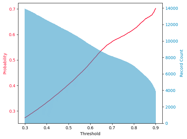
nを高くしすぎると、1位と予測する回数が減るので実際のレースに置き換えると舟券を買う回数が減ります。正答率は上がるけど、つまらない。nが低いと回数は上がるけど、正答率が下がる。n=0.8の時に正答率が60%くらいの結果になりました。
3.まとめ
LightGBMでのモデル作成とシミュレーションを行いました。精度等は特徴量の少なさとかチューニングしてないとかで大したものにはなりませんが、とても簡単に試すことができることは示せたと思います。
個人的にはpython上で特徴量を作ってモデルに入れるより、事前に特徴量はdb等に作って入れておいて出し入れをクエリで行ってpythonでの処理は学習だけにしておいた方が良いと思っています(理由は次の実践記事で)
今回の正答率は高くないですが、実際に舟券を買うときは舟券の種類や買い方も絡むので、精度をあげることだけが全てではない点が競艇予想の面白いところかなと思います。
それでは、次の記事で実際に運用を考慮したモデル作成をしていきましょう。
この記事が気に入ったらサポートをしてみませんか?