
Julia and real estate statistics

Introduction
The purpose of this article is two-fold. First I would like to introduce you to the Julia programming language. Julia is a programming language that is mostly used for computational science and data science. It has some advantages compared to other languages that are commonly used in data science like R and Python. Similar to R and Python, it is a scripting language, but it uses just-in-time compilation, making it about as fast as code written in, for example, C. As a consequence of this, many of its libraries are written completely in Julia, unlike Python and R. Another nice feature that we will use in this article, and which is often convenient for data science, is that it is easy to calculate gradients of functions using automatic differentiation.
The second purpose of this article is to show in some detail how statistical theory can be used to solve some data analysis problems that can show up in the real estate industry.
Problem
Let us begin by discussing the data and the related business problem. In our company, an important part of the business is buying and selling real estate. Having a large stock of real estate in the portfolio is costly so it is important to consider the time from a real estate is put on sale, until it is purchased by a customer, the so-called lead time. This analysis can be made complicated by looking at how this time depends on various features of the real estate or how the distribution may change over time. But here we will only look at the distribution of the lead time. In particular, we will fit a gamma distribution and use asymptotic statistical theory to test whether the distribution is exponential.
For this article, we will use some simulated data that is similar to what we observe in reality.
The gamma distribution
Let us have a look at the gamma distribution. The gamma distribution has a density function of the form
$$
p(t) = \frac{\beta^\alpha}{\Gamma(\alpha)}t^{\alpha-1}e^{-\beta t},~t>0.
$$
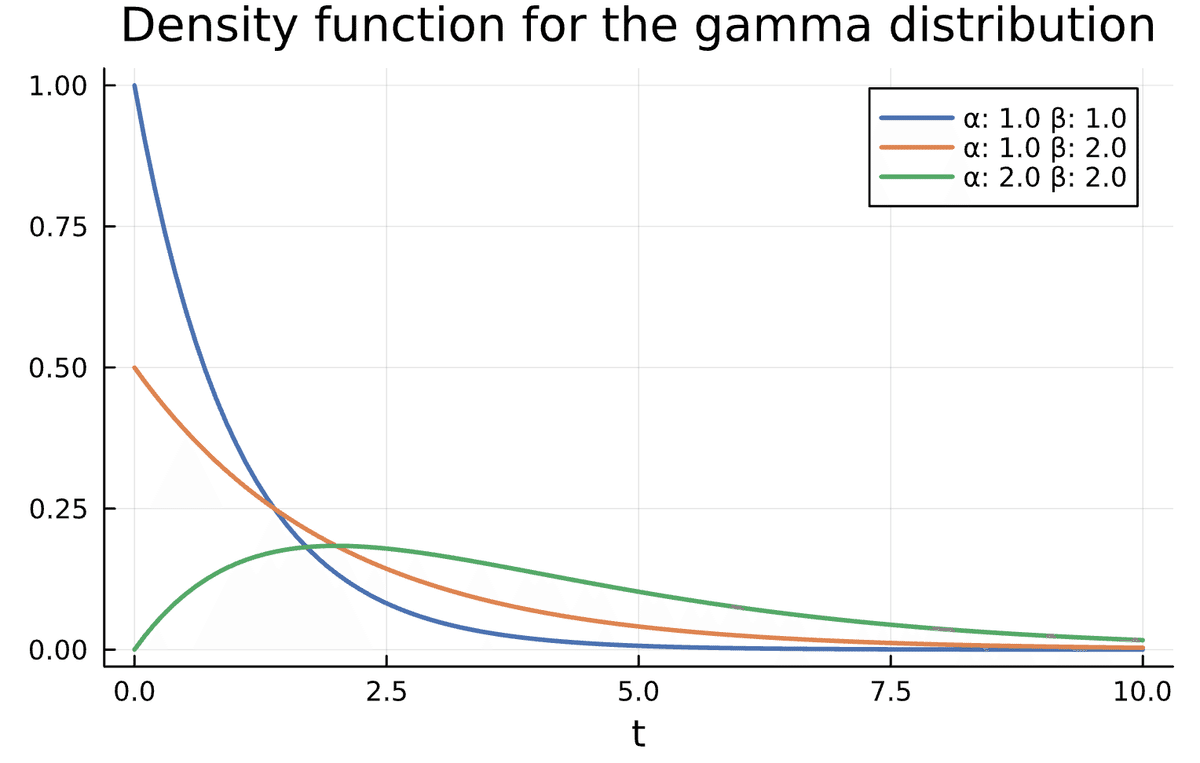
The parameter $${\alpha>0}$$ is usually called the shape parameter and $${\beta>0}$$ is called the rate. The distribution is often used to model the time until some event occurs. If we set $${\alpha = 1}$$ we get the exponential distribution, another common choice for modeling time until an event. The exponential distribution is special in that it is the only continuous distribution that is memoryless. This means that, for example, the probability that the real estate is sold the next day does not depend on whether it was just listed or if it has been for sale already for one month.
One way to quantify this is to calculate the hazard function. The hazard function, in our context, is the probability that the real estate is sold within a short time $${dt}$$, conditioned on that it was not sold at time $${t}$$. More precisely, if $${T}$$ is the time an item is sold, the hazard function is
$$
h(t)
= \lim_{dt\to 0} \frac{P(T\leq t+dt | T> t)}{dt}
= \lim_{dt\to 0} \frac{P(t < T \leq t+dt)}{P(T>t)dt}
= \frac{p(t)}{P(T>t)}.
$$
Calculating and plotting this for the gamma distribution we get figure below.
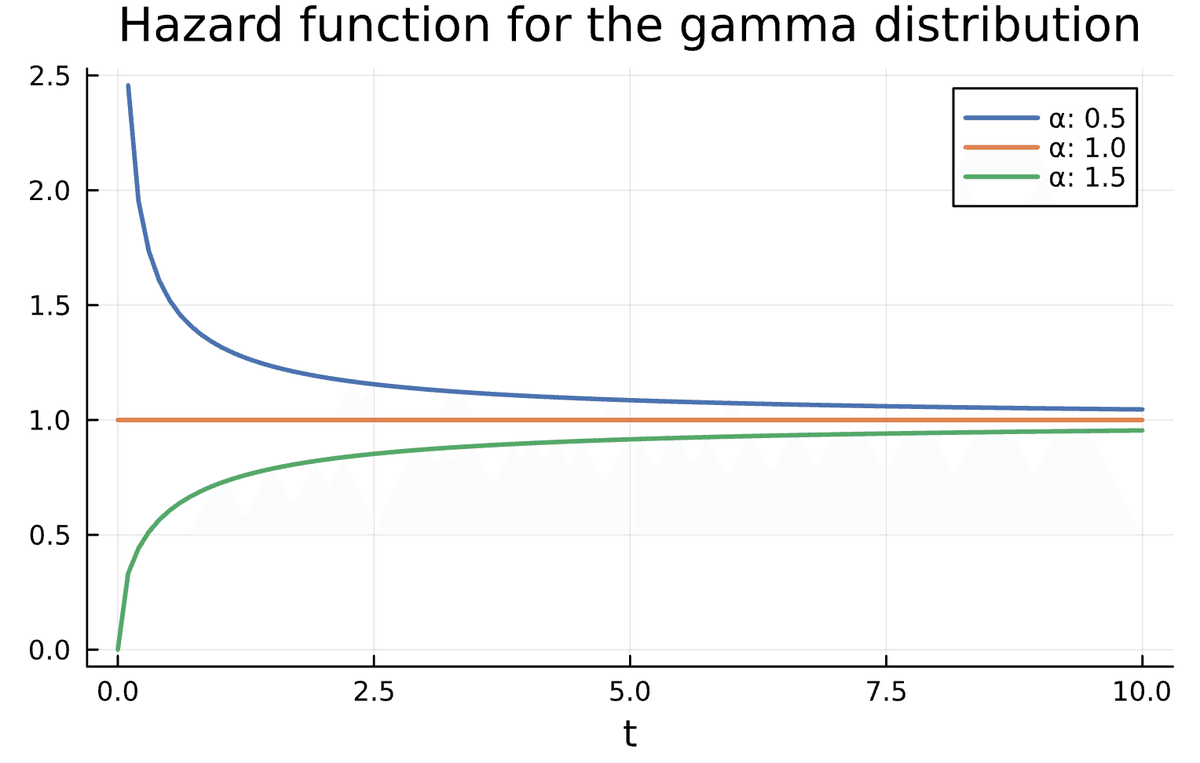
We can see that, for the gamma distribution, if $${\alpha < 1}$$ the probability of selling the real estate the next day, goes down as time passes by, and $${\alpha > 1}$$ means that the probability is increasing with time.
Data
Now let us have a look at the data. The data is in a csv file which we read using the CSV package
using CSV
df = CSV.read("data.csv", DataFrame)
Let us plot a histogram.
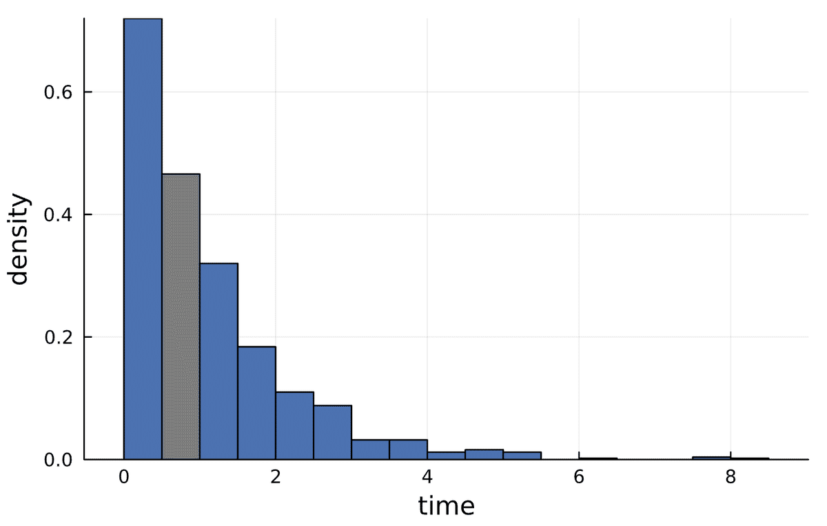
Looking at the data, the question we would like to answer is, is the exponential distribution an adequate model, or is the data generated from a gamma distribution. In other words, how does the probability of selling the real estate depend on the time it has been up for sale. To do this, let us discuss some ideas from statistical inference.
Some statistical inference
We can state our question as a hypothesis test. We would like to test $${H_0: \alpha = \alpha_0}$$ against the alternative $${H_1: \alpha \neq \alpha_0}$$. In our example, $${\alpha_0 =1}$$ i.e. an exponential distribution. We perform the test by constructing a test statistic, a function of the data, $${T(x)}$$, and a rejection region $${R}$$. That is, we will reject $${H_0}$$ in favor of $${H_1}$$ if the data $${x}$$ is such that $${T(x)\in R}$$. We will construct them such that if $${H_0}$$ is indeed true
$$
P(T(x)\in R)\leq 0.05,
$$
or some other small number. That is, the probability of making the mistake of rejecting $${H_0}$$ should be smaller than 0.05. In principle, the function $${T}$$ could be anything, but there are some common ways of constructing this function.
Let us say that we know that $${\beta = 1}$$ and then implement the log-likelihood function in Julia. To do this, we will assume that our observations are independent. This implies that the likelihood of our data is a product of the likelihood of each individual observation, and in turn the log-likelihood, by the properties of the logarithm, is a sum of the log-likelihood of each observation. In Julia this becomes.
using Distributions

function logLikelihood(param::Vector{<:Real}, x::Vector{<:Real} )
    return sum(logpdf.(Gamma(param[1],1.0), x))
end
We loaded the Distributions package which contains functions for the gamma distribution. Note that here we specified the types of the arguments to the function, however this is not necessary. The 'dot' after logpdf vectorizes the function so that it is applied to each value of x.
We then plot the log-likelihood, call it $${l(\alpha),}$$ as a function of $${\alpha}$$.
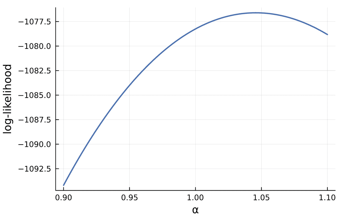
The maximum likelihood estimate of $${\alpha}$$, call it $${\hat\alpha}$$, is our best guess of $${\alpha}$$ and it makes intuitive sense to reject $${H_0}$$ if our estimate is far from the value specified by $${H_0}$$. Looking at the figure, it seems like $${\hat\alpha \approx 1.05}$$.
There are some different ways to measure the distance from $${\hat\alpha}$$ to $${\alpha_0}$$. The most obvious way is to measure distance either vertically or horizontally. In the vertical direction, we would measure the difference in the value of the log-likelihood function at our estimate and at $${\alpha_0}$$. That is we would consider $${l(\alpha_0) - l(\hat\alpha)}$$ and this would lead us to the likelihood ratio test. If we measure distance in the horizontal direction, we would consider $${\alpha_0 - \hat\alpha}$$ and this would give us the Wald test.
The test we will perform however measures distance in a third way. Since $${\hat\alpha}$$ is the value that maximizes $${l(\alpha)}$$, we know that $${l'(\hat\alpha)=0}$$. Therefore, $${l'(\alpha_0)}$$ measures how far $${\alpha_0}$$ is from $${\hat\alpha}$$. For example, if $${l'(\alpha_0)\approx 0}$$ then $${\alpha_0 \approx \hat\alpha.}$$ In summary, our test statistic will be based on $${l'(\alpha_0)}$$ and this is usually called a score test.
These three tests are asymptotically equivalent, i.e. if the sample size is large, they will accept or reject $${H_0}$$ for the same samples. Non-asymptotically they are however different and may lead to different conclusions. There is some theoretical ground for claiming that the likelihood ratio test is, in some sense, optimal. However, the Wald test has the advantage that it is easy to construct confidence intervals using it. The score test has the advantage that one does not need to calculate the maximum likelihood estimate to calculate the test statistic. In our case, all three can be used and I chose the score test simply because it contains a second-order derivate and therefore exemplifies some of the strengths of Julia.
Next, we need to construct $${R}$$ so that the probability of falsely rejecting $${H_0}$$ is not larger than the prescribed value. The log-likelihood depends on the value of the observations, which we consider random. Therefore, the log-likelihood is itself a random variable, and so is its derivative. The sum of many random variables will, according to the central limit theorem, have a Gaussian distribution, thus so does the log-likelihood. Therefore, to find the asymptotic distribution of $${l'(\alpha_0)}$$, we only need to find its expected value and variance. This is surprisingly straightforward. Let us denote the log-likelihood of a single observation $${l_X'(\alpha)}$$. Then
$$
E[l_X'(\alpha)] = \int \frac{d}{d\alpha}(l_x(\alpha))p_\alpha(x)dx = \int \frac{d}{d\alpha}(\log p_\alpha(x))p_\alpha(x)dx \\
= \int \frac{d}{d\alpha}p_\alpha(x)dx = \frac{d}{d\alpha}\int p_\alpha(x)dx = 0.
$$
In the first equality we use that the log-likelihood is the logarithm of the density of the observations, i.e. $${l_x(\alpha) = \log p_\alpha(x)}$$ and move the derivative inside the integral. In the second equality we use that, for a function $${f(\alpha)}$$, it holds that $${d \log f(\alpha)/d\alpha = f'(\alpha)/f(\alpha)}$$. The last equality uses that the integral of a density is always 1, so its derivative is 0. Using a similar calculation we can also find that the variance is
$$
Var(l_X'(\alpha)) = E[-l_X''(\alpha)].
$$
Now because the total log-likelihood is just the sum of the log-likelihood of the individual observations, so also is
$$
l'(\alpha) = \sum_{i=1}^n l_{X_i}'(\alpha).
$$
Therefore also,
$$
E[l'(\alpha)] = 0
$$
and
$$
Var(l'(\alpha)) = E[-l''(\alpha)].
$$
The quantity on the right-hand side is usually called the Fisher information, written $${I(\alpha)}$$.
With this, we have found the asymptotic distribution of $${l'(\alpha)}$$ under the assumption $${H_0}$$. Namely, after applying the appropriate scaling,
$$
l'(\alpha) \sim \mathsf N(0,I(\alpha)).
$$
Alternatively, we may write
$$
\frac{l'(\alpha)}{\sqrt{I(\alpha)}} \sim \mathsf N(0,1).
$$
The Fisher information is often difficult to calculate. However, recall from the above that $${I(\alpha) = E[-l''(\alpha)]}$$ so we may replace it with the unbiased estimate $${-l''(\alpha)}$$.
The testing procedure is then to calculate the test statistics $${s = \frac{|l'(\alpha_0)|}{\sqrt{I(\alpha_0)}}}$$ and reject $${H_0}$$ if this is larger than an appropriate quantile of the Gaussian distribution, e.g. 1.96 if testing on the 5% level. Alternatively we can calculate the p-value as $${2(1 - \Phi(s))}$$, where $${\Phi}$$ is the distribution function of the standard Gaussian distribution.
In our case, there are really two parameters but for our hypothesis test, we are only interested in one of them. To make things easier, let us assume that we know that $${\beta=1.0}$$, and get back to how to treat the case when we do not know the value of $${\beta}$$ in a follow-up article.
Statistical inference in Julia
Let us now implement this in Julia. We have already implemented the log-likelihood, so now we may calculate the gradient with respect to $${\alpha}$$ using the Zygote package.
using Zygote
gradient(x -> logLikelihood(x, df.lead_time), [1.0])([72.78165887214318],)In the next step, we find the maximum likelihood estimate of $${\alpha}$$ using numerical optimization. Note that we here also here use Zygote to calculate the gradient.
using Optimization
using OptimizationOptimJL

optf = OptimizationFunction(logLikelihood, Optimization.AutoZygote())
prob = OptimizationProblem(
    optf, [1.0],
    df.lead_time,
    lb = [0.001],
    ub = [100.0],
    sense = MaxSense
    )
sol = solve(prob, BFGS())
alphahat = sol[1]1.0457127693607415This is rather close to the value specified under $${H_0}$$. To find out how close, we now calculate the gradient and Hessian of the log likelihood function at $${\alpha_0.}$$
alpha0 = 1.0
g = Zygote.gradient(x -> logLikelihood(x, df.lead_time), [alpha0])
I = Zygote.hessian(x -> logLikelihood(x, df.lead_time), [alpha0])
The test statistic is
score = abs.( g[1]/sqrt((-I[1])))1-element Vector{Float64}:
1.7945175189982807This is close to the critical value on the 5% level. We calculate the p-value to see just how close.
pvalue = 2*(1 .- cdf(Normal(0,1),score) )1-element Vector{Float64}:
0.07273060492241501That is, we would accept the exponential distribution on the 5% level. But, since the p-value is quite small, perhaps it is best to treat the distribution as Gamma and not assume an exponential distribution.
That is all for now. Next time I would like to discuss the more complicated case of unknown $${\beta}$$.
この記事が気に入ったらサポートをしてみませんか?