Calculating 𝜋 from one random point and many circles

Good day, my name is Patrik Andersson and I work as a data scientist at AISC. At AISC we perform various kinds of research and development to support the operations of our company, GA technologies. Working as a data scientist, we use many different tools from for example statistics and computer science. One such tool that is a cornerstone in the practical use of Bayesian statistics is Monte Carlo simulations.

In its simplest form, Monte Carlo simulation uses draws of independent random numbers and the theoretical basis is then quite simple. However, in Bayesian statistics, one often uses Markov chains, that is sequences of dependent random numbers and then the theory is more complicated, using the ergodicity of the sequence to ensure its long-term properties. In this article, I will show how ergodicity can be used to calculate $${\pi}$$ in a new way. 

A Circle and a Square

A common way of introducing Monte Carlo simulation, and also it seems a not uncommon question in technical interviews, is the approximation of $${\pi}$$ using random numbers.

The algorithm goes like this: Inside a square, inscribe a circle. Pick a (uniform) random point inside the square. Repeat this many times and calculate the fraction of points that are inside the circle. As the number of points drawn grows, this fraction will then approach the ratio of the circle's area to the square's, namely $${\frac{\pi}{4}}$$.

In Python this can be implemented simply like this:

from random import uniform

inside = 0
n = 1000000

for i in range(n):
    x = uniform(0.0,1.0)
    y = uniform(0.0,1.0)
    inside += (x**2 + y**2)<1

print(4*inside/n)

The mathematical formulation of this uses the Law of large numbers which states that the average of a sequence of identically distributed independent random numbers will converge to their common mean as the length of the sequence goes to infinity.

We can write this as

$$
\frac{1}{n}\sum_{i=1}^n X_i \to \mathsf E[X_i] \text{ a.s.} \text{ as } n\to\infty,
$$

The mode of convergence here is called almost sure (a.s.) convergence. What this means is that we can construct a sequence of $${X_i}$$s that do not converge, in our case for example by drawing each point inside the circle. However, the probability of obtaining such a sequence in an experiment is 0, so we can say that the probability of the sequence converging is 1; in probability-speak almost surely.

In our case, $${X_i}$$ is either 1, if the point is inside the circle, or 0, if the point is outside. Therefore

$$
\mathsf E[X_i] = 0\cdot \mathsf P(X_i=0) + 1\cdot\mathsf P(X_i=1) = \mathsf P(X_i=1) = \frac{\pi}{4}.
$$

More Circles and Squares

I will now explain a different way of, at least in theory, calculating $${\pi}$$ by drawing only a single random point, and instead drawing many circles inside the square. I have not seen this method described anywhere else, so I believe it is a novel idea. But if you have seen it before, let me know.

The setup is the same as above, a circle drawn inside a square. We sample a point uniformly in the square and check if it is inside the circle or not. However, this time we continue with the same point. Draw four new squares inside the first square and a new circle inside the smaller square that the point happens to be in. Iterate this twice and you get something that looks like Figure 1.

Figure 1.

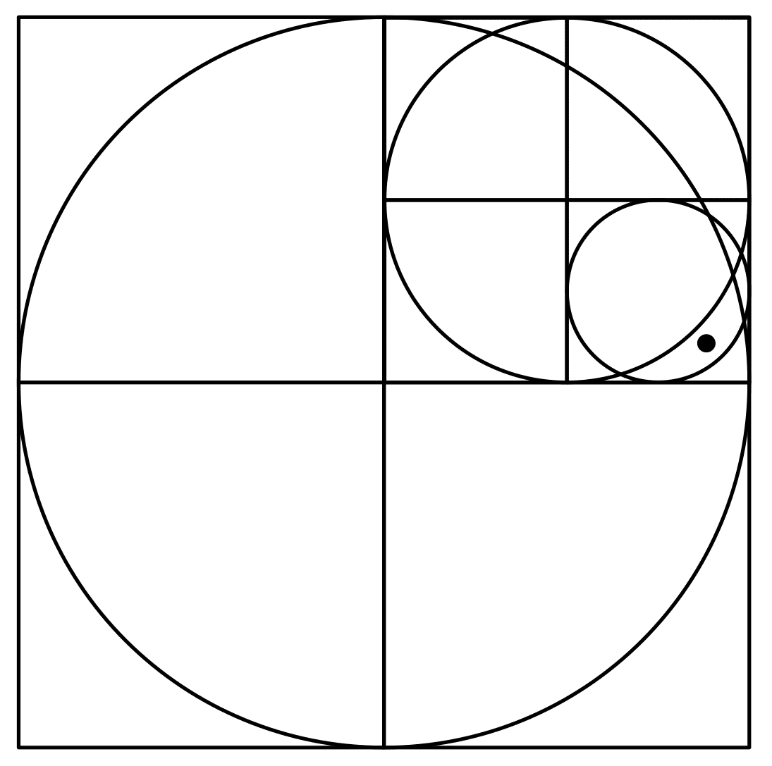
If we count the fraction of circles drawn with the point inside we get the following.

Theorem: The fraction of circles with the point inside converges almost surely to $${\frac{\pi}{4}}$$.

This is, at least at first glance, a somewhat spectacular assertion so I think it requires a proof. Let us prove it in two different ways. The first using explicit calculations and the second using more general ergodic theory.

Proof 1

To make the calculations simpler let us assume that the square is the unit square $${[0,1]^2}$$. Then, let $${C_i}$$ be the indicator for the event that the point is inside the $${i}$$th circle. We note that the $${C_i}$$s are identically distributed with $${\mathsf E [C_i]=\pi/4}$$, $${\mathsf {Var}(C_i)=\pi/4(1-\pi/4)}$$ and that the joint distribution of $${(C_i,C_j)}$$ is the same as $${(C_1,C_{j-i+1})}$$ for $${i\leq j}$$. The idea is to show almost sure convergence along a subsequence and then show that this implies convergence along the original sequence. Towards this, we calculate that

$$
\mathsf {Var}\Bigg(\frac{1}{N^2}\sum_{i=1}^{N^2} C_i\Bigg)=\frac{1}{N^4}\Bigg(N^2\frac{\pi}{4}\Big(1-\frac{\pi}{4}\Big)+2\sum_{i<j}^{N^2}\mathsf {Cov}(C_i,C_j\big)\Bigg) \\
=\frac{1}{N^2}\frac{\pi}{4}\Big(1-\frac{\pi}{4}\Big)+\frac{2}{N^4}\sum_{d=1}^{N^2-1}(N^2-d)\mathsf {Cov}(C_1,C_{1+d}).
$$

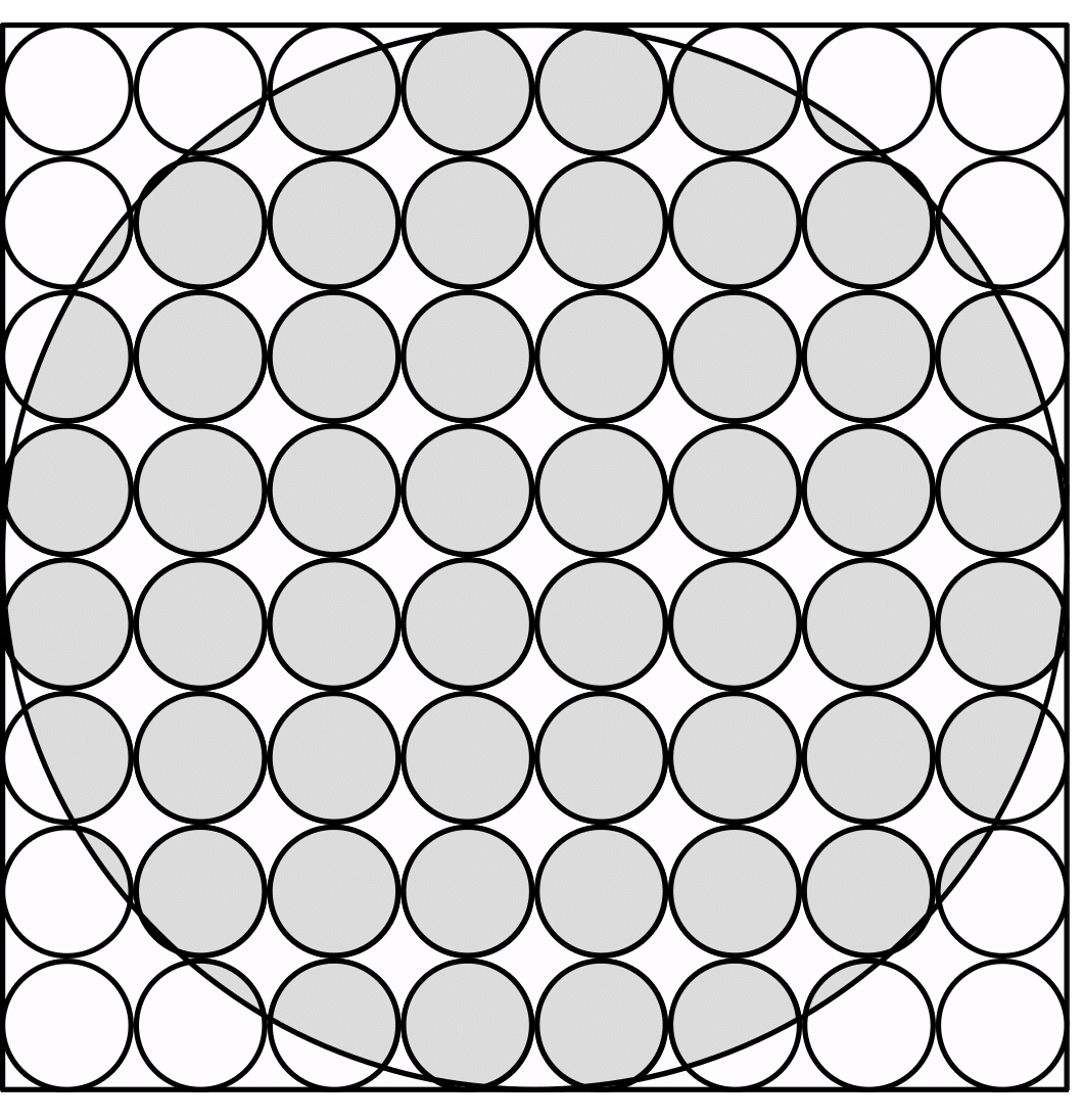
We would like to find a bound on $${\mathsf {Cov}(C_1,C_{1+d})=\mathsf E[C_1C_{1+d}]-\pi^2/16}$$. We can think of the expectation as an area in the unit square, for example in the case $${d=3}$$ the expectation would be the area of the shaded region in Figure 2.

Figure 2.

Define d-squares by

$$
\bigg[\frac{i}{2^{d}}, \frac{i+1}{2^{d}}\bigg] \times \bigg[\frac{j}{2^{d}}, \frac{j+1}{2^{d}}\bigg],~ \text{ for non-negative integers } i,j<2^d.
$$

Let $${C^{(d)}}$$ be the indicator of the smallest union of the d-squares such that $${C_1\leq C^{(d)}}$$. The number of d-squares intersected by the circumference of the large circle is less than the number of d-squares on the perimeter of the unit square, i.e. $${2^{d+2}-4}$$. We therefore get that

$$
\mathsf E\Big[C_1C_{1+d} \Big] \leq \mathsf E\Big[C^{(d)}C_{1+d}\Big]= \frac{\pi}{4}  \mathsf E\Big[C^{(d)}\Big] \leq\frac{\pi}{4}\bigg(\frac{\pi}{4} + \frac{2^{d+2}}{2^{2d}}\bigg) = \frac{\pi^2}{16} + \frac{\pi}{2^d}.
$$

Thus

$$
\bigg|\frac{2}{N^4}\sum_{d=1}^{N^2-1}(N^2-d)\mathsf {Cov}(C_1,C_{1+d})\bigg|\leq \frac{2}{N^4}\sum_{d=1}^{N^2-1}(N^2-d)\big| \mathsf {Cov}(C_1,C_{1+d}) \big| \\ \leq \frac{2}{N^2}\sum_{d=1}^{\infty} \big| \mathsf {Cov}(C_1,C_{1+d}) \big| \leq\frac{2\pi}{N^2} \sum_{d=1}^{\infty} \frac{1}{2^d} = \frac{2\pi}{N^2}.
$$

Putting this together with the above, we get that

$$
\mathsf {Var}\Bigg(\frac{1}{N^2} \sum_{i=1}^{N^2}C_i\Bigg) \leq \frac{\pi/4(1-\pi/4)+2\pi}{N^2}.
$$

From Chebyshev's inequality we then have, for any $${\varepsilon > 0}$$,

$$
\sum_{N=1}^{\infty}\mathsf P\bigg(\Big|\frac{1}{N^2}\sum_{i=1}^{N^2}C_i-\frac{\pi}{4}\Big|>\varepsilon\bigg)< \sum_{N=1}^{\infty} \frac{1}{\varepsilon}\mathsf{Var}\bigg(\frac{1}{N^2}\sum_{i=1}^{N^2}C_i\bigg) <\infty.
$$

Then by the Borel-Cantelli lemma

$$
\Big|\frac{1}{N^2}\sum_{i=1}^{N^2} C_i - \frac{\pi}{4}\Big| \to 0 , \text{ as }N \to \infty, \text{ almost surely}.
$$

Now, for any integer $${M}$$ we take $${N}$$ such that $${N^2\leq M<(N+1)^2}$$. Then, since $${|C_i-\pi/4|<1}$$,

$$
\Bigg|\frac{1}{M}\sum_{i=1}^{M}C_i - \frac{\pi}{4}\Bigg|\leq \Bigg|\frac{1}{N^2}\sum_{i=1}^{N^2}C_i - \frac{\pi}{4}\Bigg| + \frac{1}{N^2}\sum_{i=N^2+1}^{(N+1)^2}\bigg|C_i - \frac{\pi}{4}\bigg|\\ \leq \Bigg|\frac{1}{N^2}\sum_{i=1}^{N^2}C_i - \frac{\pi}{4}\Bigg| + \frac{(N+1)^2-(N^2+1)+1}{N^2}\to 0 \text{ a.s.}\textrm{ as } M\to\infty,
$$

which is the theorem.

In the second proof, we will use the concept of ergodicity. Assume we have a probability space $${(\Omega,\mathcal{F},\mathsf{P})}$$ and let $${\varphi}$$ be a measure-preserving transformation, i.e.

$$
\mathsf P(\varphi^{-1}(A))=\mathsf P(A)~\forall A\in\mathcal{F}
$$

and let $${\varphi^i=\varphi\circ\varphi^{i-1}}$$ with $${\varphi^0(\omega)=\omega}$$. Define

$$
\mathcal{I}=\big\{{A\in\mathcal{F}~|~\varphi^{-1}(A)=A\big\}}.
$$

The transformation $${\varphi}$$ is said to be ergodic if for every $${A\in\mathcal I, \mathsf P (A)\in \{0,1\}}$$. Birkhoff's Ergodic Theorem, see e.g. page 13 in Billingsley, now states that for an ergodic $${\varphi}$$ and any $${X}$$ with $${E[|X|]<\infty}$$ we have that

$$
\frac{1}{N}\sum_{i=1}^{N} X(\varphi^i \omega)\to \mathsf E [X], \text{a.s. as } N\to\infty.
$$

Second proof

Let us set our probability space as $${([0,1]^2,\mathcal B ,\mathsf P )}$$, $${\mathsf P}$$ being the uniform measure and call the event that the random point is inside the $${i}$$th circle $${C_i,~i\geq 1}$$. That is, $${C_1}$$ is the set inside the largest circle. To apply ergodic theory to our problem it is helpful to consider an alternative and equivalent formulation of the algorithm. Let $${\omega=(\omega_1,\omega_2)}$$ be the coordinates of our random point. Now, instead of drawing new circles depending on the point's position, we can transform the point. Let

$$
\varphi(\omega_1,\omega_2)=(2\omega_1~ \textrm{mod 1},~2\omega_2 ~\textrm{mod 1}).
$$

We then have that

$$
\omega \in C_i \iff \varphi^i(\omega) \in C_1.
$$

That the 1-dimensional version of $${\varphi}$$ is ergodic is shown in e.g. page 11 of Billingsley and the same arguments hold in 2 dimensions. If we let $${X(\omega)=\mathbb I_{\{ \omega\in C_1\}} }$$ we have the result that

$$
\frac{1}{N}\sum_{i=1}^{N}\mathbb I_{\{ \omega\in C_1\}}=\frac{1}{N}\sum_{i=1}^{N} X(\varphi^i\omega)\to \mathsf E[X]= \mathsf P(C_1)=\frac{\pi}{4}, a.s.
$$

Which finishes the second proof.

The second proof indicates an alternative way of looking at the algorithm. Namely, we think of our point in the square as represented by its binary expansion. The transformation $${\varphi}$$ then removes the first digit in each coordinate and shifts the rest one step to the left, thus creating a new point inside the square.