感度解析

regions = ['Hokkaido', 'Tohoku', 'Kanto', 'Chubu', 'Kansai', 'Chugoku', 'Shikoku', 'Kyushu', 'Okinawa']

import pandas as pd
import matplotlib.pyplot as plt
import numpy as np

def plot_fig1(region, csv_path):
    # Load the data from the CSV file
    data = pd.read_csv(csv_path)
    
    # Map 'Flex Load Rate' to a color gradient
    norm = plt.Normalize(data['Flex Load Rate'].min(), data['Flex Load Rate'].max())
    colors = plt.cm.viridis(norm(data['Flex Load Rate']))

    # Create a figure and axes for the plot
    fig, ax = plt.subplots(figsize=(10, 8))

    # Group by 'Flex Load Rate' and plot lines
    for rate, group in data.groupby('Flex Load Rate'):
        sorted_group = group.sort_values('DC Yearly Power Demand')
        ax.plot(sorted_group['DC Yearly Power Demand'], sorted_group[region], 
                marker='o', linestyle='-', color=plt.cm.viridis(norm(rate)))

    # Create a scatter plot with color gradient
    sc = ax.scatter(data['DC Yearly Power Demand'], data[region], c=colors)

    # Adding the color bar
    sm = plt.cm.ScalarMappable(cmap='viridis', norm=norm)
    sm.set_array([])
    fig.colorbar(sm, ax=ax, label='Flex Load Rate')

    # Set the title and labels
    ax.set_title(csv_path)
    ax.set_xlabel('DC Yearly Power Demand')
    ax.set_ylabel(region)
    ax.grid(True)

    # Display the plot
    plt.show()

# ../result 内にあるcsvファイルを探して，リストで返す

import os
def find_csv_files(directory):
    csv_files = []
    for root, dirs, files in os.walk(directory):
        for file in files:
            if file.endswith('.csv'):
                csv_files.append(os.path.join(root, file))
    return csv_files

file_list = find_csv_files('../result')
file_list

import pandas as pd
import matplotlib.pyplot as plt
import numpy as np

def plot_all_regions(regions, csv_path):
    # Load the data from the CSV file once for efficiency
    data = pd.read_csv(csv_path)

    # Create a single figure with subplots arranged in 5 rows and 2 columns
    fig, axes = plt.subplots(5, 2, figsize=(15, 30))  # Adjust the figsize as needed
    axes = axes.flatten()  # Flatten the axes array for easier iteration

    # Map 'Flex Load Rate' to a color gradient
    norm = plt.Normalize(data['Flex Load Rate'].min(), data['Flex Load Rate'].max())
    
    # Iterate over regions and axes together
    for ax, region in zip(axes, regions):
        # Apply colors based on 'Flex Load Rate'
        colors = plt.cm.viridis(norm(data['Flex Load Rate']))

        # Group by 'Flex Load Rate' and plot lines
        for rate, group in data.groupby('Flex Load Rate'):
            sorted_group = group.sort_values('DC Yearly Power Demand')
            ax.plot(sorted_group['DC Yearly Power Demand'], sorted_group[region],
                    marker='o', linestyle='-', color=plt.cm.viridis(norm(rate)))

        # Create a scatter plot with color gradient
        sc = ax.scatter(data['DC Yearly Power Demand'], data[region], c=colors)

        # Set the title and labels
        ax.set_title(region)
        ax.set_xlabel('DC Yearly Power Demand')
        ax.set_ylabel("Wind Power Generation [MWh]")
        ax.grid(True)

    # Adding the color bar on the right side of the figure
    sm = plt.cm.ScalarMappable(cmap='viridis', norm=norm)
    sm.set_array([])
    cbar_ax = fig.add_axes([0.92, 0.15, 0.02, 0.7])  # Adjust this to fit the layout
    fig.colorbar(sm, cax=cbar_ax, label='Flex Load Rate')

    # Adjust layout to prevent overlap
    plt.tight_layout(rect=[0, 0, 0.9, 1])  # Adjust the rect to leave space for the colorbar

    # Display the plot
    plt.show()

# Call the function with the list of regions and the path to your CSV file
plot_all_regions(regions,  '../result\\solar_capacities.csv')

import pandas as pd
import matplotlib.pyplot as plt
import numpy as np

def plot_all_regions(regions, csv_path):
    # Load the data from the CSV file once for efficiency
    data = pd.read_csv(csv_path)

    # Create a single figure with subplots arranged in 2 rows and 5 columns
    fig, axes = plt.subplots(2, 5, figsize=(25, 10))
    axes = axes.flatten()  # Flatten the axes array for easier iteration

    # Map 'Flex Load Rate' to a color gradient
    norm = plt.Normalize(data['Flex Load Rate'].min(), data['Flex Load Rate'].max())
    
    # Iterate over regions and axes together
    for ax, region in zip(axes, regions):
        # Apply colors based on 'Flex Load Rate'
        colors = plt.cm.viridis(norm(data['Flex Load Rate']))

        # Group by 'Flex Load Rate' and plot lines
        for rate, group in data.groupby('Flex Load Rate'):
            sorted_group = group.sort_values('DC Yearly Power Demand')
            ax.plot(sorted_group['DC Yearly Power Demand'], sorted_group[region], 
                    marker='o', linestyle='-', color=plt.cm.viridis(norm(rate)))
            #原点を通る 
            ax.plot([0, 1], [0, 1], color='black', linestyle='--')

        # Create a scatter plot with color gradient
        sc = ax.scatter(data['DC Yearly Power Demand'], data[region], c=colors)

        # Set the title and labels
        ax.set_title(region)
        ax.set_xlabel('DC Yearly Power Demand')
        ax.set_ylabel(file )
        ax.grid(True)

    # Adding the color bar on the right side of the figure
    sm = plt.cm.ScalarMappable(cmap='viridis', norm=norm)
    sm.set_array([])
    cbar_ax = fig.add_axes([0.92, 0.15, 0.02, 0.7])  # Adjust this to fit the layout
    fig.colorbar(sm, cax=cbar_ax, label='Flex Load Rate')

    # Adjust layout to prevent overlap
    plt.tight_layout(rect=[0, 0, 0.9, 1])  # Adjust the rect to leave space for the colorbar

    # Display the plot
    plt.show()

# List of regions you want to plot
regions = ['Hokkaido', 'Tohoku', 'Kanto', 'Hokuriku', 'Chubu', 'Kansai', 'Chugoku', 'Shikoku', 'Kyushu', 'Okinawa']
for file in file_list:
    try:
        plot_all_regions(regions, file)
    except:
        print(f"Error: {file}")
# # Call the function with the list of regions and the path to your CSV file
# plot_all_regions(regions, '../result/onshore_wind_supply.csv')

import pandas as pd
import matplotlib.pyplot as plt
import numpy as np

def plot_fig1(region, csv_path):
    # Load the data from the CSV file
    data = pd.read_csv(csv_path)
    
    # Map 'Flex Load Rate' to a color gradient
    norm = plt.Normalize(data['Flex Load Rate'].min(), data['Flex Load Rate'].max())
    colors = plt.cm.viridis(norm(data['Flex Load Rate']))

    # Create a figure and axes for the plot
    fig, ax = plt.subplots(figsize=(10, 8))

    # Group by 'Flex Load Rate' and plot lines
    for rate, group in data.groupby('Flex Load Rate'):
        sorted_group = group.sort_values('DC Yearly Power Demand')
        ax.plot(sorted_group['DC Yearly Power Demand'], sorted_group[region], 
                marker='o', linestyle='-', color=plt.cm.viridis(norm(rate)))

    # Create a scatter plot with color gradient
    sc = ax.scatter(data['DC Yearly Power Demand'], data[region], c=colors)

    # Adding the color bar
    sm = plt.cm.ScalarMappable(cmap='viridis', norm=norm)
    sm.set_array([])
    fig.colorbar(sm, ax=ax, label='Flex Load Rate')

    # Set the title and labels
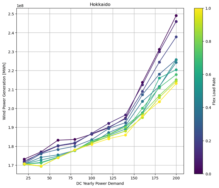
    ax.set_title("Hokkaido")
    ax.set_xlabel('DC Yearly Power Demand')
    ax.set_ylabel("Wind Power Generation [MWh]" )
    ax.grid(True)

    # Display the plot
    plt.show()

plot_fig1("Hokkaido",'../result/onshore_wind_supply.csv')

for r in regions:
    print(f"Plotting for {r}")
    for f in file_list:
        try:
            plot_fig1(r,f)
        except:
            print(f"Error in {f} for {r}")