Virus simulator

2021年3月3日 08:48

0. Background

There is a human origin book translated into Japanese below [1].
[1] Eugene E. Harris, “Ancestors in our Genome; The new science of human evolution”, (c) 2015, Eugene E. Harris; translated by Jun Mizutani, 2016 by Hayakawa publishing, Inc. ISBN978-4-15-209610-4 C0045.

On the 2nd/3rd chapter, interesting things are described. The outline is followings.
The ape that is genetically closest to humans is said to be a chimpanzee.
The branch is estimated by using genome analysis; the result is 4 ~ 6 million years ago [2].
[2] Hobolth, A., et. al. Incomplete lineage sorting patterns among human, chimpanzee, and orangutan suggest recent orangutan speciation and widespread selection., Genome Res. 21(3): 349-356 (2011).

On basis of the fossil analysis, scientists say that the period is too recent. There is also a theory that the two diverged more than 6 million years ago, then mated again 1 million years later, and finally branched at 5.4 million years ago [3].
[3] Patterson, N., et. al. Genetic evidence for complex speciation of humans and chimpanzees. Nature 441 (7097): 1103-1108 (2006).

The human population at the branched time is said to be 14,000. Based on the common sense in Today, it is surprising that the early human group was so small. Humans have been suffering from a uniquely low effective population size (the number of genetic information transmitted to offspring) for millions of years, and it seems to have compromised our immune system.
Chimpanzees, our closest relatives, are less susceptible to acquired immunodeficiency due to HIV infection, type 2 diabetes, Crohn's disease, rheumatoid arthritis, asthma, and other chronic diseases that are difficult to cure. The effective population of chimpanzees is 52,000-96,000 [3].This is induced by rare DNA mutations scattered throughout human genome [4].
[3] Retief, J., et. al. Evolution of protamine P1genes in primates, J. Mol. Evol 37(4): 426-434 (1993). [4] Lieberman, D. The story of the human body: Evolution, heath, and disease (New York: Pantheon Books; 2013).
I'm trying to express phenomenon of "herd immunity" by computer simulations based on the difference equation. The following is work reports for that objective.

1. Variables
W: world, it is fixed to be 1 (real number).
Y: amount of virus, in [Q,1-Q], where Q=small number, initial guess.
The relations between unit time is;
dY=Q*Y(0)*W(0), at time=0. The time is the integer.
Y(1)=Y(0)+dY, W(1)=W(0)-dY.
The terminal condition for the iteration is:
Y(n)>1-Q, or W(n)<Q. Such a simplified modeling is enable, because of genetic homogeneity of the human assemble.

2. Result for Q=0.05

Horizontal axis is the iterations.
Vertical left axis is values. Blue and red curves are Y(n) and W(n),
Vertical right axis is for Y(n)-Y(n-1).
The blue curve is a part of the sigmoid function, which is expected as virus increasing phenomenon.
Proof that above relation is equivalent to the sigmoid function.
The figure expresses that virus infects everyone and the phenomenon ends.
The daily derivative of the phenomenon is a yellow curve.

In above approaches, how much significance include within? Can it be represented quantitatively as truth-value/member ship-function? This is my long-terms question. Now, I am paying attention to the implication operation "A→B" based on infinite multi-valued logic. Cf. "easy Logic" article in my Note (It is a tentative one).

3. We introduce the herd immunity into the base program.
3.1 Added variable: immunity vector is Gm() in [0,1].
“Gm()=1” is that all elements have the immunity against the virus. “Gm()=0” is non immunity.
It is set with delay days “iDL=21 (3 weeks)”.
“Q” is redefined as; 0.001=1/(1+exp(-At)), t=200 as the peak day in India.
Ln(999)=-A*200, A=-0.03453. Using initial guess as Q=-A, the peak is ~160; so, we reset it, A=A/sqrt(3). Then, we get the peak t=196. The “A” is the new Q value.

3.2 Gm() Setting
At first; Gm():=0,
dY=Q*Y(0)*W(0), at time=0.
Y(1)=Y(0)+dY, W(1)=W(0)-dY, Gm(1+iDL)=Gm(0+iDL)+dY*Gp.
Gp is the percentage of people who are asymptomatic even if infected with the virus and acquire immunity. “Gp=1” means that there are same number of peoples with symptoms and those without symptoms.

3.3 Renew simulation under Gm()
dY=Q*Y(0)*Weff; where the "Weff" is,
Weff=W(0)*(1-Gm(0)), if Weff<0 then Weff=0.
Y(1)=Y(0)+dY, W(1)=W(0)-dY,
The W(0) is not a vector in section 3.2.
The terminal conditions are Y()>1-Q or W()<Q or Gm()>1.
Thus, we plot “iteration#, Y(), W(), δY(), Gm()” on a graph.

Horizontal axis is the iterations.
Vertical left axis is values. Blue and red curves are Y(n) and W(n),
Vertical right axis is for Y(n)-Y(n-1), daily patient.
The blue curve is the percentage of patients. The green line is Gm().
The Yellow curve is daily patients.
The figure expresses that herd immunity is got by assuming "immunity acquisition of asymptomatic infected persons". As a reference, the graph of Gp = 0 is shown.

4. Simulation of vaccination
The vaccine is 90% effective from 21 days after inoculation.
The vaccine start date is 65 days after the simulation start, and the end date is 180 days after the start day. The inoculation rate is even.
Viral infection continues after vaccination, and the immune effect (Gp=1) of infection is added in simulation. The result is under figure.

Horizontal axis is the iterations, elapsed days.
Vertical left axis is values. Blue and red curves are Y(n) and W(n),
Vertical right axis is for Y(n)-Y(n-1), daily patient.
The blue curve is the percentage of patients. The green and purple lines are Gm() and immune effect of vaccine.
The Yellow curve is daily patients.

---
The impact of COVID-19 on each country differs in both the number of patients and deaths. The effect of blood type is also minimal, but it exists.
It may be possible to consider the genetic differences between Europeans and Asians. To investigate them, we must go back to the past of mankind.
---
Deduced from the genome analysis of ancient apes and human bones:
1. Mankind is closely related to chimpanzees.
2. The ancestral population of humankind is small.
3. Intractable diseases are caused by the small population.

4. The Neanderthals (Homo neanderthalensis) and Denisovans (Denisova hominin) are closely related to humankind and cross with humans other than Africans.
1-4% of the Eurasian, Australoid, Native American, and North African genomes are Neanderthal genes.
Sub-Saharan Africans carry 0-0.3% of the Neanderthal gene.
Most are non-coding DNA. Neanderthal introgression would affect the human immune system.

4-6% of the Melanesian genome is consistent with that of the Denisovans.
About 1% of the genetic structure of southern China is said to be from Denisovans. A group of humans who crossed with Denisovans in the interior of Asia went south to Melanesia.

5. The Eve hypothesis deduced from the mitochondrial genome was denied.

--- Book review 1 ---
Yasuo NAKAGOME, "Even human properties are determined by the genome (in Japanese)", Kodansya, 2005.3.25, ISBN4-06-154277-X.
In p.82, followings are written.
A medical data show that many Japanese are resistant to SARS.
It is no wonder that there are such differences between races, as individual differences in the genome determine resistance to the infection.

In p.168, Gene therapy:
Modify * the DNA of a gene, which is the cause of genetic diseases.
*) Replace the base sequence of the gene with a normal one.
Replace the gene itself with a normal one.
For that purpose, "homologous recombination" is necessary.
Possible with bacteria. Homologous recombination does not occur in mammalian somatic cells.
Current technology:
Leave the broken gene as it is.
Put a normal gene in another place and let it work.

Disadvantage: Since it is not the original location of the gene, the normal regulation mechanism does not work.
Therefore, it is not possible with the insulin gene.
It is possible if the gene keeps working constantly.

The gene you want to introduce into your body:
(1) Connect to the DNA / RNA of a virus called a vector,
(2) Put it in the virus shell,
(3) Put it in the cell.

--- Book review 2 ---
Shoichi ISHIURA, "Royal Genes", Kodansha, Blue Bucks B-2099, 2019.6.20; ISBN978-4-06-516614-7.

1. Genes are present on the DNA.
2. DNA resides in the nucleus and mitochondria.
3. On the nuclear DNA, the part encoding the amino acid sequence of the protein (),
Ribosomal RNA, the portion encoding small RNA that regulates other RNA expression (),
There is a part where the base sequence repeats (microsatellite).
4. DNA testing uses the characteristics * of the microsatellite part.
* It depends on each person, and the difference indicates a parent-child relationship.
5. Maternal tracking: Mitochondrial genome, mitochondria have 37 genes.
With nuclear transplantation of fertilized eggs, there can be children with three parents, two men and women and one woman who donates mitochondria. Mitochondrial Disease; Cf. Japan Intractable Diseases Information Center, https://www.nanbyou.or.jp/entry/335
Paternal tracking: Y chromosome.
6. The blood type * is also determined by the gene.
* Differences between {A, B, AB} and O types: The O is that because a mutation in the glycosyltransferase gene makes only the 115th out of 353 amino acids. The active ferase is not produced. It can be said to be a kind of hereditary disease. The O is becoming more resistant to infectious diseases than others. But, the against function difference is only about 0.1%.

Search; "Ingman Krause Human Science", we find "The Oxford Handbook of the Archaeology and Anthropology of ...", Vicki Cummings, ‎Peter Jordan, ‎Marek Zvelebil · 2014.
Hublin, J.J. 1992. Recent human evolution in northwestern Africa. Philosophical Transactions of the Royal Society of London B: Biological Sciences 337, 185–91. Ingman, M. and Gyllensten, U. 2001.

And; we find "https://www.jstage.jst.go.jp/article/jgeography/118/2/118_2_311/_pdf". That is; Ken-ichi SHINODA, Analysis of DNA Variations Reveals the Origins and Dispersal of Modern Humans (in Japanese), Journal of Geography, vol.118（2）311~319, 2009.

現代のDNA;特に母性遺伝のミトコンドリアDNA、父性遺伝のY染色体DNA。現在、古代の人間のルートを追跡するために日常的に使用されています。
遺伝子データは実際に古代の人口移動をよりよく理解する手段を提供できるようです。
現在の世界人口のDNAパターンは、現代人が少なくとも15万年前にアフリカから出現したことを示しています。
これらの人口は、少なくとも6万年前に、アフリカからインド洋の熱帯沿岸に沿って世界の他のほとんどの地域に分散しました。東南アジアとオーストラレーシアへ。
遺伝的データは、ネイティブアメリカンの祖先がアジアの遺伝子プールから分岐し、ベーリング地峡に移動するにつれて徐々に人口が増加した新世界の開拓のモデルをサポートしています。ベーリング地峡での長い期間の後、これらの祖先は少なくとも1.5万年前に急速に南北アメリカに広がりました。
分子遺伝学的手法を使用した古代の人間の骨の検査は、過去の集団に関する遺伝情報への直接アクセスを提供します。
古代DNAの検索と分析は、現代のDNAよりも困難です。しかし、この手法は日本人の起源を推測する大きな可能性を秘めています。
縄文人、弥生人、そして現代の日本人集団の間でのミトコンドリアDNAハプログループの分布は、日本人集団の形成が人口増加の結果ではなかったことを示唆しています。
縄文人と弥生人の集団間でミトコンドリアDNAハプログループの頻度が明らかに異なることは、これらのグループの集団の歴史が著しく異なることを示しています。
しかし、どちらの人口も現代の日本人人口の形成に貢献しています。
弥生時代のアジア大陸からの東方への人口増加は、これらの人々と先住民の縄文人との混合をもたらし、現代の日本人に見られる基本的なパターンの形成につながりました。

Abstract:
Modern DNA; maternally inherited mitochondrial DNA and paternally inherited Y-chromosomal DNA in particular; is now routinely used to trace ancient human routes. It appears that genetic data can actually offer a means of better understanding ancient population movements.
The DNA patterns of present-day world populations indicate that modern humans emerged from Africa at least 150,000 years ago.
These populations dispersed from Africa to most other parts of the world at least 60,000 years ago along the tropical coasts of the Indian Ocean to Southeast Asia and Australasia.
Genetic data support a model for the peopling of the New World in which Native American ancestors diverged from the Asian gene pool and experienced a gradual population expansion as they moved into Beringia.
After a long period in greater Beringia, these ancestors rapidly spread into the Americas at least 15,000 years ago.
Examinations of ancient human bones using molecular genetic techniques provide direct access to genetic information on past populations.
The retrieval and analysis of ancient DNA is more difficult than that of modern DNA.
However, this technique holds great potential for inferring the origins of the Japanese people.
The distribution of mitochondrial DNA haplogroups among the Jomon, Yayoi, and modern Japanese populations suggests that the formation of the Japanese population was not the result of a population expansion.
Distinctively different frequencies of mitochondrial DNA haplogroups among Jomon and Yayoi populations indicate significantly different population histories for these groups.
However, both populations have contributed to the formation of the modern Japanese population.
An eastward population expansion from the Asian Continent during the Yayoi period resulted in the admixture of these people with the indigenous Jomon people and led to the formation of the basic pattern seen in modern Japanese people.

Key words：human migration, mitochondrial DNA, Y-chromosomal DNA, phylogenetic analysis, haplogroup

日本人が持つミトコンドリア DNA と Y染色体のハプログループは種類も多く，系統の大きく離れたものが混在している。
私たちの祖先が多様なルートをたどって日本へ到達したことを反映している。

We find following sentences;
There are many types of haplogroups of mitochondrial DNA and Y-chromosome possessed by the Japanese, and those that are far apart from each other are mixed. It reflects the fact that our ancestors have followed various routes to reach Japan.

島泰三、「ヒト、異端のサルの1億年」、中公新書2390,2016;　ISBN978-4-12-102390-12 C1245.
p. 204の内容：
日本人にもっとも近縁：　カムチャツカ半島基部、シベリア・イヌイット、南アメリカ、パラグアイ、グアラニ人。
第2に近縁：　シベリア・エベンキ；　バイカル湖、ブリヤート；　中央アジア、キルギス人；　南米、ワラオ人。
第3に近縁：　オーストラリア、先住民；　ニューギニア海岸民；　インド、アジア系；　南中国、少数民族。
韓国人、中国人は日本人のgroupとは異なるgroupである。

Taizo SHIMA, "100 Million Years of Humans and Heretic Monkeys", Chuko Shinsho 2390, 2016; ISBN978-4-12-102390-12 C1245.
Contents of p. 204:
Closest to Japanese: Kamchatka peninsula, Siberian Inuit; South America, Paraguay, Guarani.
Secondly related: Siberian Evenki; Lake Baikal, Buryatian peoples; Central Asia, Kyrgyz peoples; south America, Warao.
Thirdly related: Australia, indigenous people; New Guinea coasters peoples; India, Asian descent peoples; south China, ethnic minorities.
(!) Koreans and Chinese are different groups from that of the Japanese.

ニューラルネットワーク覚書：　Neural network Memorandum

35年も前のこと、back propagation algorithm of perceptron neural network という計算法があった。これは任意のvectorを、要素数の異なる別のvectorに近似的に変換する行列の直列的連結を自動生成するアルゴリズムです。必要データは2種類のvectorsである。データから変換行列を自動生成するのだからcomputer science分野では注目された。Artificial Intelligenceの黎明期の技術であって、今日学習する必要も無い、と思うが、該分野の研究をした者として、記念に書き残しておく。

Thirty-five years ago, it was known that a calculation method called the back propagation algorithm of perceptron neural network.
It is an algorithm that automatically generates multi-layered of matrices, which approximately transforms any vector into another vector with a different number of elements. The required data are two kinds of vectors.
It attracted attention in the field of computer science because it automatically generates a transformation matrix from data.
I think it's an early technology of Artificial Intelligence and you don't need to learn it today, As a person who has researched the field, I write it down as a memorial.

1.　Neural network技術記載用語の定義
入力データ　観測値を[0,1]区間の実数値にスケーリングしたvector0.
教師データ　変換後の値、[0,1]区間の実数値　vector1.
上記2種類のvector0/1の要素数は異なることを許す。
数値に単位は付かない付けられない。物理学から見れば「とんでもない」変換である。

1. Definition of Neural network technical terms
Input data "vector0" is that scaled observed values to real values in the [0,1] interval.
"Teacher data" are also converted, real value in [0,1] interval. I write it "vector1".
The number of elements of the above two types of vector0 / 1 is allowed to be different.
Numerical values cannot be attached without a unit. On the physics, it's a "ridiculous" transformation.

2. Vector0は複数のvectorsでも良い。
Vector1も複数のvectorsでも良い。
ただし、{vectors 0}-->translation-->{vectors 1}という変換に矛盾があってはならない。
データから生成される変換は1種類ということです。詳しく言うと；
{vectors 0: 観測値}-->translation-->{vectors 1: 解釈A}　です。
解釈なのだからvector 1は恣意的に定義できます。
測定値でなくとも良く、グレードI, II, III,...のようなクラス分けも[0,1]区間の数値に対応させればvector 1のデータとなります。

Vector0 may be multiple vectors. Vector1 may also be multiple vectors.
However, there must be no contradiction in the translation {vectors 0}-> translation-> {vectors 1}.
It is only one type of transformation generated from data. More specifically;
{vectors 0: Observed values}-> translation-> {vectors 1: Interpretation A}.
Since it is an interpretation as for "vector 1", it can be defined arbitrarily.
It does not have to be a measured value, and classification such as grade {I, II, III, ...} will be "vector 1 data", if it corresponds to the numerical value in the [0,1] interval.

解釈A≠解釈B、として、
{vectors 0: 観測値}-->translation-->{vectors 1: 解釈B}　と出来ます。
しかし、
{vectors 0: 観測値}-->translation-->{vectors 1: 解釈A & vectors 1': 解釈B}
とは出来ません。そういうtranslation matrixesは生成できません。
学習破綻と言います。学習とはvector0/1からtranslation matrixesを自動生成する、ことです。

As Interpretation A ≠ Interpretation B,
It can be {vectors 0: observed value}-> translation-> {vectors 1: interpretation B}.
However,
{vectors 0: Observed values}-> translation->
{vectors 1: Interpretation A & vectors 1': Interpretation B}, cannot be done.
Such translation matrixes cannot be generated.
It is called learning failure.
Again; Learning is to automatically generate translation matrixes from vector 0/1.

ゆえに、
{vectors 0: 正しい観測値}-->translation-->{vectors 1: 一部に誤りを含む解釈A}
とできます。なんとなく人の認識機能に似ているでしょう。

Therefore,
{vectors 0: Correct observations}-> translation-> {vectors 1: Interpretation A with some errors}, can be done!
Somehow it resembles a human cognitive function.

3. この行列の直列translatorの応用例
{vectors 0: 薬の物性値}-->translation-->{vectors 1: 生理的作用値}
とします。薬の有効成分の分子には電荷などの置換基が付いています。
そして様々な物性値が計測されています。薬物の動物実験により生理的な作用も分かります。
両者の物理的単位は違います。でもneural networkを使ってtranslationできます。
此処までは測定値どおしの対応づけで、得るものはありません。

3. Application example of serial translator of this matrix
{vectors 0: Physical characteristics of the drug}-> translation-> {vectors 1: Physiological action value} will do.
Molecules, which are the active ingredients of drugs, have substituents such as electric charges.
And various physical property values are measured. Animal testing of drugs also reveals their physiological effects.
The physical units of the two are different. But you can translate using a neural network.
Up to this point, there is nothing to be gained by associating the measured values with each other.

化学により新しい分子を合成できます。通常は薬として有効な既知の分子を修飾して、新化合物を作ります。その生理活性を知りたいときに、物性を測定して、このtranslatorに入力すれば、生理活性値が出力されます。それは動物実験をしなくても、生理活性値がおおよそ分かるということです。
新薬開発のために数千種の化合物を合成します。その中で有望なものを選別できる、可能性があるのです。こういう技術を構造活性相関(structure activity relationship)とよびます。

New molecules can be synthesized by chemistry. It modifies known molecules that are usually effective as drugs to create new compounds. When you want to know the physiological activity, measure the physical properties and input it to this translator, and the physiological activity value will be output. It means that you can get a rough idea of the bioactivity value without doing animal experiments.
We synthesize thousands of compounds for new drug development. There is a possibility that we can select the promising ones. This type of technology is called a structure activity relationship.

でも、化合物が細胞内に浸潤して複雑な反応の連鎖の結果が生理的作用です。そういう詳細を、対象化合物群すべてに共通のもの、としているのがこのtranslationですよね。
ゆえに「予測精度が悪いだろう」と思います。事実そうなのですが、何千もの化合物の動物実験はできませんし、費用も莫大、時間もかかります。では何で化合物を選別します？

However, the result of a complex reaction chain in which a compound infiltrates into a cell is a physiological action.
It is this translation that makes such details common to all target compound groups.
Therefore, I think that the prediction accuracy will be poor. As is the case, animal testing of thousands of compounds is not possible, costly and time consuming. So why select compounds?

参考までに、構造活性相関の実務上の見解です。以下引用：
ーーー
M. Yoshida, MD said that:
微生物からのスクリーニングは，時として予想外の大きな発見をもたらす。
真菌の形態異常を惹起する抗生物質、レプトマイシンがある。
タンパク質核外輸送因子の発見と抗がん剤開発を可能にしたユニークな天然物である．
レプトマイシンの標的として同定されたCRM1 は，真核生物共通のタンパク質核外輸送因子であった。
さらにCRM1 は骨髄腫をはじめ多くのがんで重要な役割を果たすことが明らかになった。
現在，注目を集めるがんの分子標的の一つとなった。
微生物が作る化合物の多様性は，その標的分子の多様性につながる。作用機序解明は新発見をもたらす。
真菌にのみ特異的な増殖阻害と形態変化を誘導する物質としてレプトマイシン（LM）A/Bがある。
構造は分子末端にδ-ラクトン環を有する不飽和脂肪酸である。
レプトマイシンは酵母に20 ng/mLという低濃度で増殖停止とともに形態伸長を引き起こす、特徴を示した。
動物細胞にもnMオーダーで細胞周期のG1期停止を誘導する。さらに抗腫瘍活性を示す。
構造活性相関から，末端の不飽和のδ-ラクトン環は活性に必要である。
一方、末端にあるカルボン酸は不要であることが示唆された。
実際に，カルボン酸に種々の化学修飾をしても活性は維持される。
飽和のラクトンを変換すると、活性が完全に失われる．
LMの発見の後，カズサマイシン，アンギノマイシン，レプトールスタチンなどいくつかの類縁体がいずれも強い抗腫瘍活性物質として報告されている。

Screening from microorganisms sometimes leads to unexpectedly large discoveries.
There is leptomycin, an antibiotic that causes morphological abnormalities of fungi.
It is a unique natural product that has enabled the discovery of protein nuclear transport factors and the development of anticancer drugs.
CRM1, identified as a target for leptomycin, was a protein nuclear transport factor common to eukaryotes.
Furthermore, CRM1 has been shown to play an important role in many cancers, including myeloma.
It has become one of the molecular targets of cancer that is currently attracting attention.
The diversity of compounds produced by microorganisms leads to the diversity of their target molecules. Elucidation of the mechanism of action brings new discoveries.
Leptomycin (LM) A / B is a substance that induces growth inhibition and morphological change specific to fungi only.
The structure is an unsaturated fatty acid with a δ-lactone ring at the end of the molecule.
LM was characterized by causing growth arrest and morphological elongation in yeast at a low concentration of 20 ng / mL.
It also induces G1 phase arrest of the cell cycle in animal cells on the order of nM. Furthermore, it shows antitumor activity.
From the structure-activity relationship, the terminal unsaturated δ-lactone ring is required for activity.
On the other hand, it was suggested that the carboxylic acid at the end was unnecessary.
In fact, the activity is maintained even if the carboxylic acid is subjected to various chemical modifications.
Conversion of saturated lactones results in complete loss of activity.
Following the discovery of LM, several analogs such as kazusamycin, anginomycin, and leptolstatin have all been reported as strong antitumor actives.
ーーーココまで引用　End of quoting

4. この行列の直列translatorの応用例(II)
このNoteでは、薬物の構造活性相関はやりません。
今、世界はSARS-CoV-2のCOVIDパンデミックで大変ですね。各国でPCR検査陽性者(cases)と死者(deaths)統計値が集計されています。それらは統計サイトで編集され一般に公開されています。
そのデータ間の相関をtranslatorで調べてみましょう。

4. Application example of serial translator of this matrix (II)
On the Note, I do not correlate drug structure-activity.
Right now, the world is having a hard time with the SARS-CoV-2 COVID pandemic. PCR positive cases and deaths statistics are aggregated in each country. They are edited on the statistics site and made publicly available.
Let's examine the correlation between the data with a translator.

U.S.のcases/deaths間のtranslatorを生成し、それにU.K.のcasesを入力すると、U.S.社会のCOVIDに対するresponseによるU.K.のdeaths変化が出力されます。それはU.K.のdeathsとどう違うのでしょうか？災害に対する社会のresponseの相違が数値的に表現できる可能性がある、と思いませんか？

If you generate a translator between U.S. cases / deaths and enter U.K. cases into it, the U.K. deaths change due to the response to the COVID of the U.S. society will be output. How is it different from U.K.'s deaths? Don't you think there is a possibility that the difference in social response to a disaster can be expressed numerically?

5.　日本のCOVID-19
確認計算：　Perceptron type, 3 layer neural networkの非線形fitting function.

<PCNNxor9.png> 9値論理のexclusive OR学習の結果です。全81ケースで正常に学習しています。

COVID計算：
[1]　日本のCases/Deaths data の関係をneural networkに学習させます。
データ期間：　2020.2.21~2021.9.20, down loaded from Our data in the world, master data.
入力データ： Ln(cases)+線形関数+ニューロン・バイアス
教師データ： Ln(deaths)
中間層neuron数：13個
学習関数：　1/2層シグモイド関数(eps=0.25)、2/3層線形関数(eps=0.1)
過学習防止：　10k毎にerasing
学習回数：　60k

<OrgDataJapan.png>　元データです。Cases(black), Deaths(Red)
このデータをneural networkに入力できるように、次のように変形します。
NN用のスケーリング：　入力データを[0.1,1]区間にスケーリングする。教師データを[0,1]区間にスケーリングする。
Cases/Deaths間の遅延を減らすために、両者の距離を最小化する。
こうして得られたNN入力、教師データです。

<NNinData.png>このデータで60k回学習した結果です。Cases-->Deathsの関係を学習しています。

<NNRs.png> erasingにより中間層のニューロン数が12個に減少しました。
この結果は入力データに線形関数が入っています。何故入れたのかというと、日本のCOVID対策が「実施された」からです。
統計的に有意なのはワクチン接種でしょう。その線形関数を除いてNNを学習させます。

<LackLinear.png>グラフの右端でNNの出力(青)とdeaths dataの数(赤)が離反しています。
日本のCOVID対策が「実施されなければ」deaths curveは青線のようになる、ということをNNは示しています。
ワクチンが重症化を防止する、と言われていますが、この計算はそれを支持しています。

NNに入力した線形関数の働きについての考察：
線形関数はNNの内部で任意の点で折れ曲がった線分の働きをします。
線形関数を入力して、教師データに折れ曲がった線分値をして学習します。

<mNNlinearBent.png> Learning=25k, data#=1000, NN=(Lenear+bias,10,1),
erasing per 3k. 折れ曲がり点は任意です。教師データで（自動的に）指示できます。
ワクチン接種の有効性が出る期日が不明でも、教師データ(deaths values)に反映されればokです。

COVIDはもう1.5年間も蔓延しています。その間に治療法の改善も成されています。それはcases数とdeaths数の全般的な勾配に現れます。その効果も線形関数で取り入れています。

6. 考察　学習アルゴリズム
6.1　Neural network内の情報の流れ
入力データを行列形式 0<X(i,n)<1 で表記します。区間[0,1]にするためにscalingが済んでいるとします。
Index "i"は1事象を表すベクトル。"n"は事象を識別する番号。
3層のneuronから成る3段Neural networkは2個の行列で表されます。
1,2層のneuron間を繋げる第1行列を U(i,j) とします。
添字"i"はX(i,n)と共通です。添字"j"は第2層のneuronに対応します。
2,3層のneuron間を繋げる第2行列を V(j,k) とします。
添字"j"は第2層のneuronに対応します。添字"k"は第3層のneuronに対応します。

Neural network内で情報は次のように流れます。
X(i,n)-->1st neurons-->*U(i,j)-->2nd neurons' operation-->*V(j,k)
--->3rd neuron's operation-->output value, indexed by "k"
この流れが"n"だけ繰り返されます。ゆえにoutput行列はOut(k,n)です。
U(),V()の前に"*"記号が付いるのはU,V行列値が乗算され、かつ添字i/jについてΣを取る、ことです。
Σにより全"i"が1個の第2層neuronに入力されます。第3層neuronについても同様。

Neuron's operation: Σの結果をxと書くとき、sigmoid(x)=1/{1+exp(-x)} これがoperationです。
以上を式で書くと、
x(j)=Σi X(i,n)*U(i,j); 2nd neoron's (j) output=1/{1+exp(-x(j)}=H(j).
y(k)=Σj H(j)*V(j,k); 3rd neoron's (k) output=1/{1+exp(-x(k)}=Out(k,n).
添字"n"がX()とOut()にだけ付いています。
Neural networkは、入出力パターン数に依存しない関数です。

6.2　Back propagation algorithm
このOut()を目的の値になるように2行列U(),V()を決定するのが学習です。
その方法をback propagation algorithmと言います。

目的の値をTE(k,n)と書きます。0<TE(k,n)<1.
最初U(i,j),V(j,k)は不明ですので、一様乱数値とします。　-0.3<U(i,j)<+0.3 とします。
当然、Out(k,n)≠TE(k,n) です。ここで、1つの"n"値について以下のようにします。
δ(k)=Out(k)-TE(k), Δ(k)=δ(k)*[Out(k)*{1-Out(k)}], Err=Σk δ(k)**2,
∂V(j,k)=-ε*Δ(k)*H(j); V(j,k)+∂V(j,k)-->new V(j,k).
"ε"はパラメータ、学習係数です。ε~0.3です。Out(k)*{1-Out(k)}部分はsigmoid関数の微分形です。

第2層の誤差は、
δ(j)=Σk V(j,k)*δ(k), Δ(j)=δ(j)*[H(j)*{1-H(j)}] です。
∂U(i,j)=-ε*Δ(j)*X(i); U(i,j)+∂U(i,j)-->new U(i,j).

誤差が第3→第1層へ逆方向に伝搬している、イメージなのでback propagation (BP)という名称がつきました。
以上の操作を添字"n"について全部行います。
そうするとErr（スカラー、値）はErr(n)というベクトルになります。

以上の計算を最初から繰り返して　Err(n)~0 vector　とします。BPは一種のiterationです。
0 vectorならば全入力について目的値になった、ということで、学習完了です。

6.3 考察
BPは完了するalgorithmなのでしょうか？いいえ、必ず完了するとは限りません。
第2層のneuron数の決定法がalgorithmに無いでしょう。ゆえに、
1st/3rd layer's neurons >> 2nd neurons　とすると完了しません。
また、矛盾のある入力・教師データ、
X(i,n)＝X(i',n)　を　TE(k,n)≠TE(k',n)　とすると、同じものから違ったものへ投影する、ことになり矛盾となり完了しません。

論理関数　AND/ORの学習は完了が容易ですが、exclusive ORはなかなか完了しません。
2次元空間での線形分離は容易ですが、非線形分離は容易ではないです。
多値、多次元空間になればなるほど[0,1]区間の細かい部分まで分離しなければならないので完了に至るitaration数は多くなります。

第2層のneuron数の決定法がalgorithmに無いので、
2nd neurons >> 1st/3rd layer's neurons とすると、どうなると思います？
その場合は完了はします。教師データについてはokですが、未入力の

X(i, new_n)につぃて問題が出てきます。
今、X(i,n1), X(i,n2), X(i,n3)のときTE(i,n1)<TE(i,n2)<TE(i,n3)とします。
X(i,n2), TE(i,n2)を学習しないneural networkに、X(i,n2)を入力して（neural networkで推測する）、Out(i,n2)~TE(i,n2)が得られるか？というと、あまり好ましい結果にはなりません。汎化機能不十分と言います。
Neural networkの応用で重要なのはこの汎化機能です。
未学習のデータについても「妥当な」結果を得る、必要があるのです。

汎化機能には必要最小限の第2層ニューロン数でneural networkを構成する必要があります。そのためにerasingという操作をします。

Erasing: If{|U(i,j)|<0.1}then U(i,j)=0、V(j,k) についても同様。
注意点：　BP処理とは独立です。この操作をすると、Err値が大きくなります。ゆえにiteration毎に行っては「学習できません」。
経験的には1k~10k毎に行います。小さな学習破綻をまれに繰り返しながら、ゆっくりとBPでErr値を小さくします。

行列要素値0とは、neuron層間の結合を切る、ことです。
すると前の層からの情報が無くなるneuronも出てきます。
そういうneuronの出力は添字"n"に依存しない定数です。
それはbias値として次の層のneuronに全て作用します。

Sigmoid関数S(x)の微分形はS(x)*{1-S(x)}です。
S(0)=0.5, S'(0)=0.25, maximum of {S'(x)}　なので、bias neuronが存在しても問題ありません。
学習を高速化する働きもあります。
この意味で、第1層の1 neuronを{X(i,n)}から独立したbias neuronとして付加させることがあります。
私の経験として： Bias neuronは1個付加させるべきです。

学習高速化について、次の点も留意します。
(1) 第1,2層間のU()を変化させる式、
∂U(i,j)=-ε*Δ(j)*X(i); U(i,j)+∂U(i,j)-->new U(i,j)
を見ましょう。入力データX(i)が乗じられています。X(i)=0のとき∂U(i,j)=0です。
すなわち入力値0の近傍は学習しにくいです。
従って、入力データのscalingは[0.1,1]区間とすべきでしょう。最小値0.1としたのは、この値を大きくすると、
学習完了のためにU()の精度を高く計算するデメリットが生じるからです。

(2) U(),V()を変化させる式の値は定数εで小さくされています。
これを大きく ε>0.5とするとErr→∞となって学習破綻します。
"n"の数が大きくなるほど εを小さくしてください。ただし ε<0.1は薦めません。

(3) Sigmoid関数の引数xにについて：
|x|>5.0ではS'(x)~0となって、実質、U(),V()が変化しません。
それで|x|>5.0でも5.0として計算します。こうすると3%ぐらいは変化できるので悪影響を小さくできます。
状況によっては5→2.5でも良いとおもいます。ただし非線形分離機能は低下します。
Neural networkはBP法の表には出ない、こういうparameter値により「性能」が変わります。

(4) 第3層のneuron operationのバリエーション
これまで、それはy(k)=Σj H(j)*V(j,k); 3rd neuron's (k) output=1/{1+exp(-y(k)}=Out(k,n).
ですのでSigmoid関数です。しかし、微分可能な関数ならば、それに置換してもかまいません。
y(k)=Σj H(j)*V(j,k); 3rd neuron's (k) output=y(k)=Out(k,n),
故に、
δ(k)=Out(k)-TE(k), Δ(k)=δ(k)*1, Err=Σk δ(k)**2,
∂V(j,k)=-ε*Δ(k)*H(j); V(j,k)+∂V(j,k)-->new V(j,k) です。
このようなneural networkは非線形分離機能が低下しますが、時系列変化を良く表します。
急激な変化を再現しませんが、逆にそれは長所、たとえば推測精度向上になります。
以下、この形の3層neural networkについて述べます。

7. Neural networkを使った推測値
7.1 学習完了したneural networkで推測することが可能である。
ここで述べる推測の定義：
学習に用いた{X(i,n)}とは異なる{X(i,m)},n≠mからOut(k,m)を計算する。
条件：　添字"i"について対応を取ること。

1<n<Nなる順序づけができる時系列データの場合、1<m<N なら内挿、1<N<mなら外挿である。

推測計算はX(i,m)をneural net {U(i,j),V(j,k)}に入力しOut(k,m)を計算する。
X(i,m)は測定値が「ある」。当然のように思われるだろうが大事なことである。
測定値が無い推測はあり得ない、と考えられるか？測定値に誤差がある、ときはどうか？
このようにFuzzy性を考えると、「当然」は簡単には取り扱えない。
この問題は奥が深いので、まずは、X(i,m)が正確な測定値とする。

X(i,m)をneural networkに入力するとき、学習順序集合{1,2...n,...N}と、
入力値mの順序関係を守らなければならない。
例　{1,2,...,m,...N}とする。
{1,2,...,m-1}の順にBP計算して"m-1"位置までの{U(i,j),V(j,k)}を更新してからX(i,m)を入力する。

Neural net {U(i,j),V(j,k)}は定数の行列ではなく、
[{U(i,j),V(j,k)}n; TE(k,n)]と表記すべきindex "n"についてのiterative matrixである。
誤差ベクトルErr(n)も{Err(k,n); TE(k,n)}である。

では　X(i,m)→{U(i,j),V(j,k)}→Out(k,m)　と推測値を計算したとき、
{TE(k,n)}集合にOut(k,m)を追加する必要はあるか？
それは「必要なし」とされている。ゆえに、誤差ベクトル{ERR(n)}は推測操作により不変である。
Out(k,m)は測定値ではなく、neural networkが推測した値であるので、誤差ベクトル不変、は必要である。

時系列データとは言えない「薬物の生理活性：QSAR」をneural networkで行う場合；
1<n<Nなる順序づけができない。その場合はBP学習をrandomな順序で行う必要がある。そして誤差ベクトル{Err(n)}は、{X(i,n)}集合の全要素のBP学習が終わった後で、
{U(i,j),V(j,k)}行列更新部を除いたforward方向だけの処理で計算する。
その場合は学習回数が多くなる。
また第3層のneuron operationを線形関数からSigmoid関数に戻す必要がありうる。薬物の種類によりQSAR用のneural networkの線形・非線形の度合いが異なる。

外挿の場合を考察する。簡単な例をあげ、それに沿って考察する。
例：　{X(i,n)}={0,1,2,.....N}={x}, TE(k,n)}={f(x)}　線形関数から非線形なf(x)を生成するneural networkを学習する。
入力要素：　線形値{x}＋bias(=constant 1)
教師データ：　{f(x)}
第3層neuron's operation 線形関数
データscaling 入力[0.1, 0.9], 教師[0, 0.9]区間。区間最大値を1→0.9とする。

この場合NNの作用は；
目的関数を第2層のneuron operation, Sigmoid functionの線形結合で近似する、処理と等価になる。
外挿であるから{X(i,m)}={N+1,N+2,...}={x'}を入力する。Scalingは学習期間と同様。
第1層neuronには0.9以上の値が入ってくる。
X(i,N+p)→NN→Out(k,N+p); p={1,2,....}.
出力集合{Out(k,N+p)}に誤差は、（一般的に）定義できない。
モデル計算ならば、{x+p}→f(x+p)が計算できる、から
各TE(k,N+p)について、
δ(k)=Out(k)-TE(k), Δ(k)=δ(k)*[Out(k)*{1-Out(k)}], Err=Σk δ(k)**2,
∂V(j,k)=-ε*Δ(k)*H(j); V(j,k)+∂V(j,k)-->new V(j,k).
以下　U(i,j)も同様。
とBP処理できる。誤差計算部だけに止め、外挿の有効範囲を調べることもできる。

各TE(k,N+p)について、TE(k)~Out(k),iteration-1　と考えてiterationについてself-consistency(SCF)としても良い。
SCF処理により外挿期間の延長をめざす。

モデル計算：　時系列データの欠測部をNNで補間した例
Learning iter=28k, data#=1000, NN=(Lenear+bias,7,1), erasing per 5k.
defect data zone: 500±25 and 750±25, total defect#=102 data.
全データの10%が欠測です。

<DefectLout.png> 青細線がNN outputs、黄緑太線がTeaching dataです。
欠測部は0出力です。average{ERR(n)}=1.52E-6, max{ERR(n)}=1.40E-4.
Erasingで{U(),V()}のうち5経路が0となりました。
学習は欠測部を除いて完了しています。

欠測部をNNで補間します。Teaching dataが欠測部には無いので、
iteration#が1つ前のNN outputで代用します。

<DefectInterpol.png>　青細線がNN outputs、黄緑太線がTeaching dataと
補間されたNN出力値です。average{ERR(n)}=1.63E-6, max{ERR(n)}=1.40E-4.
折れ曲がる点の前後が欠測となる悪条件ですが、妥当な補間です。
直線増加部分の補間は完全です。

8．データと雑音、補間精度
今まで、入力・教師データには「雑音が無い」としてきました。
しかし、QSARの実務で、そのような都合の良いデータはありません。
必ず雑音が含まれています。そのとき、NNはどのような学習となるのでしょうか？AIの教科書に記載が少ないので、ここで実例を示します。

例：　Learning iter=28k, data#=1000, NN=(Lenear+bias,7,1), erasing per 5k.
defect data zone: 500±25 and 750±25, total defect#=102 data.

{X(i,n)},{TE(k,n)}データに0.8を乗じ、|uniform random number|<0.2を加算します。
0.1<|X(i,n)+uniform #|<1となるようなuniform#を選びます。
同様に|TE(k,n)+uniform #|<1.

ゆえに、欠測＋雑音20%の入力＆教師データでBP計算をします。
結果：

<RealQSARL.png> 青細線がNN outputs、黄緑太線がTeaching dataです。
欠測部は0出力です。average{ERR(n)}=2.01E-2, max{ERR(n)}=0.226.
Erasingで0となった経路はありません。

max{ERR(n)}を見ると学習完了ではありません。
しかし、これ以上iterationしても、この値は小さくなりません。
Erasingできない、ということはNNの構造が「雑音を学習できない」ことを暗示しています。
しかし、雑音には有意な情報が無いので、学習できないことは、好ましいことです。
この学習未完了のNNで補間します。
補間部のteaching dataは無いので、1つ前のiterationのOut(k)で代用します。

<RealQSARdP.png> 青細線がNN outputs、黄緑太線がTeaching dataです。
average{ERR(n)}=2.01E-2, max{ERR(n)}=0.226.
補間部では線形増加が見られません。
data # [550,1000]区間での回帰直線を示します。

<RealQSAR_R.png>　青点NN outputs、黒線が回帰直線です。
傾き=0.0016 (期待値 0.0020)です。

9. データと雑音、外挿精度
外挿も補間と同様です。Neuronの値が[0,1]区間なので、学習用のデータはscalingを[0.1, 0.9]区間のように小さくしてください。外挿できる範囲が[0,1]区間に制限されています。

例： Learning iter=28k, data#=800, NN=(Lenear+bias,7,1), erasing per 5k.
{X(i,n)},{TE(k,n)}データに0.8を乗じ、|uniform random number|<0.2を加算します。
0.1<|X(i,n)+uniform #|<1となるようなuniform#を選びます。
同様に|TE(k,n)+uniform #|<1. Scaling=[0.1,0.9].
0<n<801で学習して800<m<1025を外挿します。その結果：

<ExtraPol.png> Data# 1~800が学習、入力と教師データ（薄緑）の20%の乱数が含まれます。青線はNNの出力値です。学習期間でもrandomに揺らいでいます。
Data# 801~1025が外挿期間です。Neuron出力値<0.93まで妥当な外挿です。
外挿時もNNにデータを入力します。その範囲が<0.9となっている*ために、外挿が0.93で止まっているように見えますが、本来は1まで外挿可能です。

*　20%乱数を付加するので<1には出来ません。外挿時の入力にも乱数を付加しています。もし乱数付加をしない、のなら外挿を1まで延長できます。外挿期間は教師データは1つ前のdata#のNN出力です。
NNの外挿は1 step predictionのように見えますが、NNの出力を使っているので、1 step predictionではありません。

1次関数の外挿ではない場合、NNにデータを入力する前処理のところで「線形化」してください。高精度の外挿を実行するために必要です。線形化関数が不明な場合は、線形化用のNNを検討してください。

10, Parameter ε 制御
6.2節で学習algorithmにparameter εを導入しました。
>>その部分を引用>>
目的の値をTE(k,n)と書きます。0<TE(k,n)<1.
最初U(i,j),V(j,k)は不明ですので、一様乱数値とします。　-0.3<U(i,j)<+0.3 とします。
当然、Out(k,n)≠TE(k,n) です。ここで、1つの"n"値について以下のようにします。
δ(k)=Out(k)-TE(k), Δ(k)=δ(k)*[Out(k)*{1-Out(k)}], Err=Σk δ(k)**2,
∂V(j,k)=-ε*Δ(k)*H(j); V(j,k)+∂V(j,k)-->new V(j,k).
"ε"はパラメータ、学習係数です。ε~0.3です。Out(k)*{1-Out(k)}部分はsigmoid関数の微分形です。
>>ココまで>>
ε=0ならばV(j,k)=new V(j,k)で学習しません。εの値により学習の度合いを制御できます。
ε → ε*L(js,j0,je; J)　と変更しdata number "J"の関数とします。
L()関数のdefinition:
S(x)=1/{1+exp(-x)}, -3<x<3; ~S(x)=1-S(x).
L(js,j0,je; J), const: js<j0<je, J=argument.
if(J<js) L(J)=~S(-3);
if(js<J<j0) L(J)=~S(x), x=-3*(J-j0)/(js-j0);
if(j0<J<je) L(J)=~S(x), x=3*(J-j0)/(je-j0);
if(je<J) L(J)=~S(+3).
Thus, 0.9526>L(J)>0.0474

J<js ならば定数~εの学習です。
J~0　で学習強度1/2、　J>jeでは5%未満の学習機能です。
こうして、時系列データの指定期間だけを「強調」学習します。

長期間にわたる時系列データ(1年以上の測定など)では初期の頃と末期の状況が変わり、説明変数(descriptors)の作用が異なることがあります。
そういう場合に、parameter ε 制御を行います。実例を示します。

COVID-19のPCR検査陽性者数C(i)と死者数D(i)をNNで関連づけます。
{D(i)}は{C(i)}の部分集合なので、そういう関連は（非線形でしょうが）可能です。
[{C(i)}+bias neuron]--->(NN)--->{D(i)}.　ここでindex "i"は時系列を表します。
しかし、この関連では「人間の社会的行動の何が有効に働いたか？」が分かりません。
そこで、人間の社会的行動とは何だろう？と考え、それを推定します。一種の予測で、説明変数(descriptors)の推定です。
[{C(i)}+bias neuron+Descriptor1(i)+Descriptor2(i)]--->(NN)--->{D(i)}.
というNNを学習します。

{C(i)}はすでにウイルスを体内に持っている者の集合なのだから、人間の接触機会などがdescriptorではありません。蓋然性のあるのは医療関連の行動でしょう。治療法、ワクチン普及による抗体保有者の比率です。
これらを時系列descriptorsとして関数で表現します。
我々は、
{Descriptor1(i)}, Linear function {1-x(i), i=1,2,.......N}, 0<x(i)<0.9,
{Descriptor2(i)}, Fully vaccinated person's ratio for the population, {Vcc(i)}, 0<Vcc(i)<1.
を採用します。このdetaはワクチンが有効な抗体を作り出す期間(21days)分シフトさせます。

Descriptor1が奇妙に思われる、かも知れません。
COVIDには現在、これと言った効果のある（インフルエンザのタミフルやリレンザのような直接的にウイルスを叩く）治療薬がありません。パンデミック以来1.5年経過してもそうです。
しかし既存薬を組み合わせた療法は漸進しています。
それが死亡率を漸減させます。その効果を 1-x という直線で表します。
以上、NNの入力データを示します。

<COVIDjpDT.png> Shifted*-Cases(Blue), Deaths(Red purple), Vaccination(Green). *) Using minimize the distance between Cases and Death data. Left vertical axis is Ln(numbers/d) scale, Right one is Ratio for the population.

これらをNN用にscalingして線形関数とbiasを追加して学習させます。
3 descriptors+1 bias; iter=20k, erasing per 1000 times;
ε=0.25(for U()), ε=0.1(for V()), js=430, j0=460, je=490; hidden layer's neuron=5. Input neuron=4, Output neuron=1.

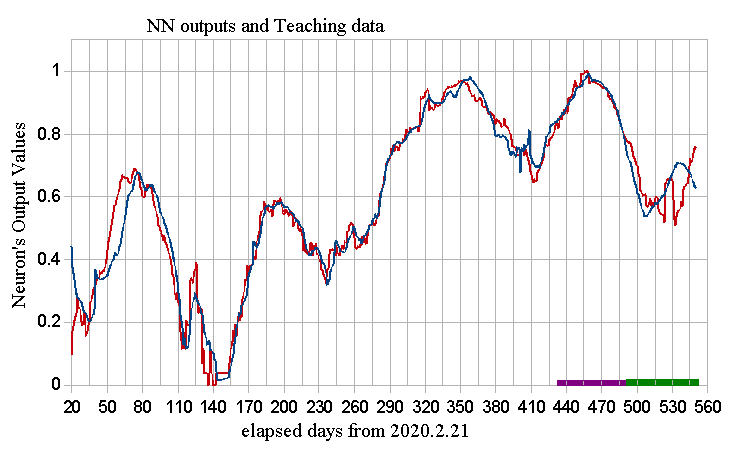
<COVIDjpVcc.png> NN output values (blue), Teaching data (Deaths)
Bold lines of purple/green are the period of L()-function (week Learning).
説明変数3を使うと、弱く学習しても教師データの再現性は良好です。
次にVacctination's descriptorを無効にします。Descriptor 2のinput neuronとU()の結合を切ります。その時のNN出力です。

<COVIDjpNoVcc.png>
青線のNN出力値が教師データよりも有意に大きくなります。
ニューロン出力値では実際の数との関係が明確ではないので、Scalingを逆関数で元の自然対数値に戻し、さらに指数関数で測定値に戻します。
そうして経過日455~551days期間の、「ワクチン接種なしのときの予測死者数」と「現実の死者数」をグラフに描いてみました。

<COVIDjpVeff.png> NNは「死者数減少」については「ワクチンの有効性」を示しています。

11. 時間軸の関数化
時系列dataは等間隔の時刻毎の測定値です。測定していない時刻の現象については何も情報を持っていません。これが情報学の見解です。

本sectionでは、それを崩し「現象は突然に変化しない」という仮定の下、
補間が有意として議論を進めます。断っておきますが、その仮定が成立しない現象（たとえば、株価予測など）には適用不可。

物理化学の測定と解析では；　測定値そのもの(X(i))より、自然対数値を使用します。 {X(i)}→{Ln(X(i))}。
時刻"i"の近傍の時刻では、測定値が正規分布する、と考えられるでしょう。
分布値をLn()スケールでプロットすれば二次関数です。

3測定時刻{xm, x0, xp}とLn()を取った測定値{ym, y0, yp}があるとき、
未測定時刻の現象値（以下めんどうなのでLN()を省略）は、二次関数で補間します。

変換：　測定値→二次関数
ym=Axm**2+Bxm+C, y0=Ax0**2+Bx0+C, yp=Axp**2+Bxp+C;

ym-y0=A(xm**2-x0**2)+B(xm-x0), (ym-y0)/(xm-x0)=A(xm+x0)+B,
y0-yp=A(x0**2-xp**2)+B(x0-xp), (y0-yp)/(x0-xp)=A(x0+xp)+B;

(ym-y0)/(xm-x0) -(y0-yp)/(x0-xp)=A(xm-xp),

∴A={(ym-y0)/(xm-x0) -(y0-yp)/(x0-xp)}/(xm-xp).
B=(ym-y0)/(xm-x0)-A(xm+x0).
C=ym-Axm**2-Bxm.

二次関数f(A,B,C; x)→補間値、期間 (xm+x0)/2 < x < (x0+xp)/2.
極は 2Ax+B=0, x=-B/(2A).　期間内に存在すれば極あり、存在しないならば「不明」。この補間で離散時刻の測定値を連続測定値へ変換します。両端では測定期間が短くなります。ここは、Computer解析なので1/10の離散間隔で代用します。

普通、時刻は等間隔に取る（samplingする）ので、{t0,t1,...tn}, 0<{ti}<1　と書きます。
t(i)=dt*(i), i={0, 1, 2,...n}, dt=1/n　-->　Y(t)~1*t, 0<t<1.　t(i)は離散、Y(t)は連続。
0<Y()<1. "~"とは連続関数の離散点で右辺のように定義される、こと。

この直線関数のように離散点で定義されたY()を、
値でdt間隔に0から増分方向に切り出した数列が、離散時刻index "i"です。

ゆえに、時間は増分方向に進み、後戻りしない、という性質が付与されています。かつY()を定義する関数は単調関数に限定されます。

dt=1/n, t(i)=exp{dt*(i)}-exp(0), --> Y(t)~exp(t)-1, 0<t<1.
このY(t)についてもdtで切り出した、new index "i"が存在します。
この新"i"で1/10の離散間隔の関数値を引用して現象を見ると、
時刻間隔の次第に短くなる事象に見えます。
逆にいえば、時間軸方向に現象を拡大して見る、ことになります。
exp()を考えるのはこの議論の背景に拡散的な現象を考えているからです。

例：　f(x)={sin(x)+1}/2, 0<x<2π　をnew index "i"={0,1,...n}で表示する。
n=999. 離散点数999+1-2=997.

<DPexp0.png>　元のdataはf(x)={sin(x)+1}/2, 0<x<2π　を'old' index "i", dt=1/nで等間隔samplingした有限ベクトルです。
2次式の補間*処理により段差を生じることなく、現象の時間方向の拡大が成されています。
*)上記の式は、現象の微分形が計算できないとき、
現象の極に漸近する近似的な手段として利用できます。.......Eq.(11.0)

これで準備が出来ましたので、本sectionで目指す予測を示します。

<DPexp2.png>　dt=2/n, t(i)=exp{dt*(i)}-exp(0), --> Y(t)~exp(t)-1, 0<t<2,
f(x)={sin(x)+1}/2, 0<x<4π.
問題：　index 2~270 の測定値（関数値）から271~998期間の値を予測する。1周期分の測定から次の周期を予測する。拡散的な現象であるとする。

まず1周期分の測定から、
dt=z/n, t(i)=exp{dt*(i)}-exp(0), --> Y(t)~exp(t)-1, 0<t<z,........Eq.(11.1)
のzを決めます。
z-value, distance*
-------------------------
1.52, 0.01194
1.62, 0.0097
1.72, 0.00732
1.82 0.00481
1.92 0.00218
2.02 0.00055
2.12 0.00336
2.22 0.00622
2.32 0.0091
2.42, 0.01198
------------------------
* It is defined by "DPexp2.png & Learning term" and "Eq.(11.1)".
Using z={1.92, 2.02, 2.12}, {0.00218, 0.00055, 0.00336} and "Eq.(11.0)", we get;
pole=2.00046, value=0.00047.
約1/1000の精度で結果を得ます（期待値2）。このpole値で1周期分のデータから次周期を予測します。

<DPexpRs.png>　pole値が真値2より大、かつ両端で期間が短くなるので、
次周期より短く予測されています。予測精度は妥当です。
波の性質さえ分かっていれば、このような長期の予測もできます。

時間軸方向にズレる関数はneural networkではうまく近似できないので、
QSARとは関係が少ないですが記載しました。

---------------------------------------------------------------------------

私の目的：
計測データだけから将来を推論したい、少なくとも現状を把握したい。
しかし、現実はそう甘くなく、普通はできません。
それで、何らかの結論に関係しそうな「現象」の時間変化量を探します。
COVID解析で言えば、生物、医学的な個別の指標でない、たとえば、治療技術全般の進歩などです。
対症療法といえども、症状の進行を遅らせれば、その間に体の免疫機能がウイルスに勝ち、回復に向かう可能性がある。
こういう「漠然とした効果」は、集団として長期間、継続観察・計測して、データ数が多くならないと利用できませんが、そいう効果を結果に結び付けたいのです。

My objective:
I want to infer the future from measurement data only, or at least grasp the current situation. However, the reality is not so easy and usually NOT possible to do so.
Therefore, we look for index of time variation of the target "phenomenon" that seems to be related to some conclusions.
On COVID analysis, we accept that it is not a biomedical individual indicator; for example, advances in therapeutic technology in general medicines.
Even with symptomatic treatment, if the progression of symptoms is delayed, the body's immune function may overcome virus and recover.
Such "vague effects" cannot be used unless the number of data is large after continuous observation and measurement as a group for a long period of time, but I would like to link those effects to the discussions for taget phenomenon.

小生のブログ　https://scienceimg140e.fc2.net/
COVID, 9/18の記事の図をクリックして拡大して見てください。
この図では死亡率を患者数（青）に乗じて、赤の死者数と比較できるようにしています。
2020年の春頃（左側）は各国で赤線が青線の上に来ています。（現在に比べて）死亡率が高い、ということです。
G7諸国では治療法の進歩がみられます。
治療法の内にはワクチンの接種率や、罹患者増による集団としての抗体誘導効果（俗にいう集団免疫）も含まれます。

I have a blog: https://scienceimg140e.fc2.net/
Click on the figures in the "COVID, 9/18" article to enlarge them.
In those figures, the mortality rate is multiplied by the number of patients/cases (blue line) and compared with the line of deaths in red.
Around the spring of 2020 (on the left), the red line is above the blue line in some countries.
It means that the mortality rate is high (compared to the present).
We found some advances in treatment in the G7 countries.
Among the treatment methods are vaccination rates and;
It also includes "antibody-inducing effect" of human due to the increasing in number of affected people (so-called herd immunity).

12. 　試論：日本,UK, Brazil, India, RussiaのCOVID死者数とワクチンの相関
1)　ワクチンの種類は国順に；
ファイザーmRNA, アストラゼネカ・チンパンジー・アデノウイルス・ベクター、各種、各種、スプートニクV・アデノウイルス・ベクター方式です。
2)　相関は教師付き3層ニューラルネットワークで行います。
Neurons are {4,5,1} for each layer.
DescriptorはPCR陽性者数、線形関数、ワクチン・2回接種者の人口比率の3種です。
Teaching dataは死者数です。Bias neuronを付加します。
各々1 neuronに対応します。

3)　データをNNに入力するための前処理
PCR陽性者数と死者数は期間内で数値積分して、係数（＝致死率）をPCR陽性者数に乗じます。
PCR陽性者数と死者数の自然対数をとります。
両者のpeakがズレています。時間軸方向にPCR陽性者dataをシフトさせます。日本21日、UK 23、Brazil 0, India 13, Russia 10 daysです。
そして[0.1,1]と[0,1]区間にscalingします。

線形関数は治療法の進歩に対応するのでf(x)=1-x, min{f(x)}=0.1とします。

ワクチンの抗体誘導期間を21日とします。抗体は240日で半減するとします。ワクチン接種率も「死者数を減少させる要因」として導入しているので、1.0から率を減じた関数をdescriptorとします。本データに限りscalingしません。

4)　Simulation
period: 2020.2.21~2021.9.18
data source: https://github.com/owid/covid-19-data/tree/master/public/data/
Data on COVID-19 (coronavirus) by Our World in Data.

Neuron's operation: Hidden layer, 1/{1+exp(-x)}, x=ΣU(i,j)descriptor(i), for the period. If |x|>2.5, then x=2.5*sign(x).
Output layer: x, x=ΣV(j,k)Hidden neuron(j), for the period.
以上、本NNでは非線形性を「低く」とっています。完全に線形ならば重回帰分析です。非線形・重回帰分析というapproachも存在しますが。
Learning iterations=10k, Erasing per 1k.です。過学習には配慮しています。

Learning後、ワクチンのdescriptorのみを無効化してiterativelyに結果をNNから引き出しますが、このとき、ワクチン接種率0.1%以上から後の期間のε値を4%以下にします。
実質的にback propagation (BP)せずにNNをforward 方向にだけ動かします。
これをやらないと、異なるdescriptorsの場合のBPが働きはじめ異常な結果となります。

5)結果と考察

<NNan0928A.png> NN入力・教師データ

<NNan0928B.png> ワクチン接種効果図
青：ワクチン接種なしの時の死者数、NNの出力値。
赤：報告死者数、NNの教師データ値。
青線が赤の上ならば、効果あり（図のA領域）。下ならば逆効果（B領域）。
逆効果の原因：　ワクチンを絶対的なCOVIDバリアと誤解して、無節操な行動を取ると、感染→重態→死、となります。

本Simulationでは治療法の改善効果が入っています。その分、ワクチンの効果が低く計算されます。
インド、ロシアではワクチンの効果は、死者数で見る限りありません。
原因：インドではワクチン接種率が低い。ロシアのスプートニクVは、ベクターの一部にアデノウイルス5を使用しています。このウイルスには抗体を持った人がいます。そうするとベクターが働かず、コロナウイルスの抗体ができません。

本稿は「試論」段階のものです。これから検証に入ります。　記、2021.9.29.

13. Verification

14 Verification 2: Fourier transformation approach
The wave phenomenon can be decomposed into spectra by Fourier transform.
The COVID phenomenon (changes of cases, deaths per a day) is a diffusion phenomenon, but if it diffuses in a closed system, it will converge. In case of one type of virus, it is represented by the sigmoid function.
However, due to human collective behavior (lockout, etc.) and viral mutations, it is done by multiple sigmoid functions. In such a case, a part of the apparent phenomenon intensity seems to be a wave phenomenon.
Let's find out if the consideration is true or an illusion.

(1) Pretreatment of the phenomenon
The COVID phenomenon cannot be Fourier transformed as it is. Pretreatment is required.
Process 0: Linearization of exponential growth phenomenon by natural logarithm
Process 1: Introduction of periodic boundary conditions
Process 2: Removal of tilt
Process 3: scaling to [0,1] interval

(2)　Cases of {Japan, Russia, UK, US, Brazil, India}

<FrIntensity.png> Fourier spectra for {Japan, Russia, UK, US, Brazil, India}
If the gradient is 0, the phenomenon is converged.

If the intensity of high frequency waves is strong,
<1> The virus that causes the wave has a "function to suppress reproduction". Its function is not the biological property of the virus itself; It is a society-response characteristic of the human infected with the virus. It depends on the country.

<FrCasesJpRu.png> Frequency and the intensities; in case of Japan/Russia.

<FrCasesJpRuRs.png> Observed and Fourier transformed Cases.
Japan: Using 24 waves, to test the precision of Fourier transformation.
Russia: Using 6 waves; to test the accuracy about large intensity waves until 6th ones.

14. Verification 3: Differential form of Sigmoid function: Sigmoid関数の微分形
Sigmoid function, f(x)=1/{1+exp(-x)},　は対象微生物の餌に上限がある「閉鎖系」での個体数の時間変化を表す関数です。一般化して、
S(x)=1/{1+exp(-αx)}, (d/dx)S(x)=αS(x){1-S(x)}, -∞<S(x)<∞, α=scalar constant.
COVID解析では、無限大まで利用しません。ピーク位置から1/2~1/4の範囲で使用します。計算の利便性のため、
S(x)=1/{1+exp(-x)}, (d/dx)S(x)=S(x){1-S(x)}=S'(x), -2<S(x)<2,
とします。
COVIDのcases, deaths数の時系列変化曲線は、何の対策も打たなくて、かつ
SARS-CoV-2ウイルスが変異しなければ、S'(x)となります。
本節はSigmoid関数の微分形を調べます。

Sigmoid function, f (x) = 1 / {1 + exp (-x)};
It is a function that expresses the time change of the number of individuals in a "closed system" where the food of the target microorganism has an upper limit. We generalize it as,
S (x) = 1 / {1 + exp (-αx)}, (d / dx) S (x) = αS (x) {1-S (x)}, -∞ <S (x) <∞, α = scalar constant.
COVID analysis does not use up to infinity. Use in the range of 1/2 to 1/4 from the peak position.
For convenience of calculation;
S (x) = 1 / {1 + exp (-x)}, (d / dx) S (x) = S (x) {1-S (x)} = S'(x), -2 <S (x) <2,
will do.
The time-series change curve of the number of cases and deaths of COVID does not take any measures, and
If the SARS-CoV-2 virus does not mutate, it will be S'(x).
This section examines the differential form of the Sigmoid function

(1) S'(x)概形
(d/dx)S(x)=S(x){1-S(x)}=S'(x), -2<S(x)<2　をExcelでプロットします。
この形状は正規分布、Gaussian, G(x)=Nexp{-α(x-μ)**2}, に類似しています。
μ=0, α,N値を変えてfittingします。

<Sigm1009A.png> {S'(x), Gaussian, the difference}
α=1, S'(x)のpeak値は0.25です。Gaussianのα=0.217, N=1/4.
-2<S(x)<2、有効数字2ケタならば　S'(x)=G(x)　と見なして問題ないでしょう。両者の相関 y=0.990x+0.0047, R2=0.999.

注意：Gaussianとdirrerential Sigmoidは異なる関数です。範囲-10<x<10、自然対数表示でしめします。

<Sigm1013.png> 両者を同一視できるのは-2<x<2 or |Ln(Δy)|<3.5です。狭い範囲でも、同一とみなせる、ことが重要です。
S'(x)のLn()表示で、裾野部分が直線に漸近しています。これは感染初期のcases per dayのプロットが、指数関数的で、Ln()表示すると「直線」である、という事実を証明しているのです。

Gaussianの自然対数は二次関数です。ゆえに2次回帰分析によりsigmaod微分関数の極値が分かります。ということは、積分形のSigmoid関数の最大漸近値＝「将来の」cases値の収束値が分かるのです。

この事実を利用してインドのcasesデータをGaussian近似する。

データの回帰分析式：
第1波：期間31~360 elapsed days, start day=2020.2.21.
F(x)=-0.000158x**2+0.0722x-1.251; R2=0.965, on Ln() scale.
第2波： 390~500 elapsed days, same start day.
F(x)=-0.000859x**2+0.765x-161.862; r2=0.932.
Another expression: F(x)=-0.00118x**2+1.0451-222.879, R2=0.981, 420<x<480.

R2値の大きさから、インドではSigmoid関数の最大変化点(209 day)と値(9.3万人)である。
R2が0.5のような小さい値であると上記の値に信頼性がない。
以上から計算される第1波の積算感染人口 968.3万人、全人口の0.70%である。
積算はelapsed day 31からpeak day 209まで数値積分して、その2倍を計算する。
これが、本論から導出される第1波の感染人口である。以下、同様に第2波でも計算する。
第2波の計算開始日は360 elapsed day（第1，2波のbottom）である。

結論：　これでは集団免疫にはならない。実際、第2波が起こった。
しかし！何故このような小値でCOVID第1波は収束に向かったのでしょうか？
インドの14億人の集団は不均一な集合で、200×2=400daysの期間では；
小さな部分集合体として機能（準閉鎖系）していることになります。

第2波：　最大変化点(443 day)と値(39.1万人)である。Mutationによる、新集合体の出現と考えられる。このような大きな変異がコロナウイルスで発生するとは2020年の段階では考えられていなかった。
この件については、Research Center for Advanced Science and Technology, the University of Tokyo　のProf. T.KODAMA, MD.が適切なPDF資料をnetに公表されておられる。検索して熟読されたい。

計算される第2波の積算感染人口 2044万人、全人口の1.5%である。
結論：　集団免疫にはならない。変異株が出現すれば、第3波もあり得る。

2021.10.14のworldmeters: https://www.worldometers.info/coronavirus/
ではIndia, total cases=34,019,641, new cases=+19,141 である。
このNoteの第1，2波解析での合計感染者数は9/18時点で、968+2044=3012万人　1.9*26=49万人, ∴3061万人なのでorderとしては妥当である。

次の検証として；　準閉鎖系の微分方程式を考察する。
Indiaの第2波の終焉(~2021.7.14)以後もcases=0へ指数関数的に収束せず、
cases数が横這いになっている。準閉鎖系のゆるやかな「拡大」が起こっていることを、示す。

「準」の意味は、期間を限れば、差分方程式:
Q0: initial world space, Q(i): world at "i"-step,
Y0: initial case, Y(i): cases number at "i"-step,
A: increment constant (scalar > 0) for Y(),
B: increment constant (scalar > 0) for the world.

discrete differential EQ,
dY={Q(i)/Q0}A*Y(i)*dt, Y(i+1)=Y(i)+dY;
Q(i+1)=Q(i)-dY+B.
が近似的に成立する、ことです。この方程式系の動きをsimulationで調べます。
Parameter {Y0,A,B,Q0}={0.1, 0.1, 0.1, 10}で110stepまで計算した結果です。

<DiffModeL1.png> Green: the world of virus growth, Blue: cases, Red: differential cases. This is the result of solving the considered viral replication using finite difference equations using model parameters. We tried to reproduce the case of 2nd wave in India.
準閉鎖系のゆるやかな「拡大」ということが、simulation上では再現できる。以上、Sigmoid関数の微分形の考察から、演繹可能な状況を述べました。　　記　2021.10.14

準閉鎖系についての試行計算：
日本のCOVID-19, cases dataの日変化曲線は波打っています。この波は有限フーリエ変換によれば、3.63か月周期の第4波のintensityが最大です。微分・シグモイド曲線のピーク値付近はGaussianですが、Gaussianを同変換すると、第1周期の波が最大となります。
集団免疫が成立しているのなら、cases曲線はSigmoid関数となるので、
日本のcases曲線は「集団免疫が成立していない」ことを示しています。

何故、3~4か月周期の波が存在し得るのか？を準閉鎖系差分方程式により追跡します。
波が複数あるので、準閉鎖系も複数でなければなりません。複数の系は相互に干渉しています。その干渉は、人流によるウイルスの輸送がもたらしています。
人流dataは市販されていますが高価です。残念ながら採用できません。Netに在るのは都道府県の第二次dataです。差分方程式に使えそうな物は在りませんでした。それではmodel計算するしかありません。

ここでは3準閉鎖系の相互作用modelを考えます。
{shell 1}⇔{shell 2}⇔{shell 3}
(1) specification of shell 1:
Q0: initial shell space, Q(i): space at "i"-step,
Y0: initial case, Y(i): cases number at "i"-step,
A: increment constant (scalar 0.1) for Y(),
B: increment constant (scalar 0.3) for the space.
descreat differential EQ,
dY={Q(i)/Q0}A*Y(i)*dt, Y(i+1)=Y(i)+dY;
Q(i+1)=Q(i)-dY+B*exp{B0*(i-imax0)}.
Setting parameters: A=0.1, B=0.3, Q0=10, Y0=0.1, dt=0.1, imax0=180,
if i<imax0 than B0=Ln(0.5)/90,
if i>imax0 than B0=Ln(0.5)/180.

(2) specification of shell 2/shell3:
Q02: initial shell space, Q2(i): space at "i"-step,
Y02: initial case, Y2(i): cases number at "i"-step,
A2: increment constant (scalar 0.1) for Y2(),
B2: increment constant (scalar 0.3) for the space.
descreat differential EQ,
dY2={Q2(i)/Q20}A2*Y2(i)*dt, Y2(i+1)=Y2(i)+dY;
Q2(i+1)=Q2(i)-dY2+B2*exp{B02*(i-imax2)}.
Setting parameters: A2=0.1, B2=0.3, Q02=10, Y02=0, dt=0.1, imax2=273/362,
if i<imax2 than B02=Ln(0.5)/90,
if i>imax2 than B02=Ln(0.5)/180.
Interaction between space 1/2:
Z02=Y(i)*1.e-4, Z20=Y2(i)*1.e-4
Y(i)=Y(i)+Z20-Z02, Y2(i)=Y2(i)-Z20+Z02.
The interaction is done per "it; mod=10".
In case of shell3, Q02-->Q03, Q2()-->Q3(), dY2-->dY3,....
Z23=Y2(i)*1.e-5, Z32=Y3(i)*1.e-5,
Y2(i)=Y2(i)+Z32-Z23, Y3(i)=Y3(i)-Z32+Z23.

We get a following result.

<DiffMDL4.png>

15. Verification 4: 2層の線形NNによる説明変数の寄与simulation:
Test: 三角関数の線形結合の係数をsampling dataから求める。
フーリエ変換するのが一般的であるが、ここでは線形NNで解く。
問題：
descriptor 1: y=0.1+{sin(t)+1}*0.45, 0<t<2π, 0.1<y<1.
descriptor 2: y=0.1+{cos(t)+1)*0.45, same,
descriptor 3,4: y=0.1+{sin(2t)+1)*0.45, y=0.1+{cos(2t)+1}*0.45,
descriptor 5,6: y=0.1+sin(t/2)*0.9, y=0.1+{sin(3t)+1}*0.45.
teaching vector: T={sin(t)+sin(2t)/2 +1.5}/3.
data sampling: 1k points.
これを、以下のNNでBP法で解く。
NN=(7,1), Learning iter.=20k, eps=0.05, erasing per 2k.
BP error: 0.000001.
結果：
We get following descriptor contribution.
d1: 0.6623, sin(t)
d2: -0.0034, cos(t)
d3: 0.3301, sin(2t)
d4: -0.0013, cos(2t)
d5: -0.0026, sin(t/2)
d6: 0.0003, sin(3t)　妥当な解である。精度は2桁である。
The contribution is changed under the BP-iteration; That is;
BPはiterationの性質もあるので、係数がiteration毎にどう変化して、解に至るかがわかる。
図で係数の変化を示す。

<NNLNtest.png> The above table is got at the iteration end point.
Those are acceptable. The NN has a reasonable function.
精度良い解を得るには1周期分のdataが必要である、ことを本図が示している。
COVID dataにこのような「1周期」という概念は無いが、
「解を得るために」十分なdataかどうかの判定はしなければならない。
多くの議論で、この観点からの再検証が求められる。
------ End of the Test --------

補足：　NNは入力ベクトル(descriptors)を教師ベクトルに非線形に対応づける。
この対応を定量的な「量」として求める。
そのために、descriptorを非線形に変形する部分と、
変形されたdescriptor vectorを線形にteaching vectorに対応させる部分とに分離する。
ゆえに「線形NN」と称していても、処理全体を通して見れば「非線形変換」である。
そもそもBPでteaching vectorとの差異を繰り込んでいるので非線形である。

問題 (Test 2)：
descriptor 1: y=0.1+{sin(t)+1}*0.45, 0<t<4π, 0.1<y<1.
descriptor 2: y=0.1+{cos(t)+1)*0.45, same,
descriptor 3,4: y=0.1+{sin(2t)+1)*0.45, y=0.1+{cos(2t)+1}*0.45,
teaching vector: T=[{sin(t)+sin(2t)/2 +1.5}/3, 0<t<2π; {sin(t)/2+sin(2t) +1.5}/3, 2π<t<4π],
data sampling: 1k points.
途中で目的の関数形が変化する。この場合のdescriptorsの係数はどうなるのか？
これを、以下のNNでBP法で解く。
NN=(5,1), Learning iter.=2k, eps=0.05, erasing per 200.
BP error: 0.00023, teaching vectorが変化しなければO(-6)である(確認済)が、変化するとO(-4)となる。
iter回数は2kであるが20kとしても同じである。

結果：
We get following descriptor contribution.
d1: 0.4606, sin(t)
d2: -0.0252, cos(t)
d3: 0.4729, sin(2t)
d4: 0.0412, cos(2t)
全期間の平均はsin(t):sin(2t)=1:1である。NNはそれを計算している。
NNの出力値の変化を示す。

<NNLNtest3.png> 　R2=0.997
この結果からdescriptorsの、期間に依存する線形結合であるteaching vectorを、BPの計算法で得る2種類の解が存在する（精度O(-4)で）。
予期しなかった別解のdescriptorsの値の変化を示す。

<NNLNtest3A.png> d1~4値はiteration中、変動する*。ここが線形重回帰分析との相違である。
*)R2値もiteration中0.990~1.000間を変動する。

--------- 補足　終----

We use the NN, and analyze COVID data of Japan.
The NN output (blue) and the teaching data (deaths, red) are,

<NNLNcovidJP.png> The BP error are 0.0026, iter# is 20k.　線形NNでも精度よく日本のCOVID, deaths曲線を、{cases, linear-function, Vaccination} dataから計算できる。本simulationは重回帰＋1 step prediction approachである。Descriptorは：The input data are following descriptors;
d1: Cases data, natural Logarithm, scaling in [0.1,1].
d2: Linear decreasing function, in [1, 0.1].
d3: full-Vaccination data, in [1, 0.1]. である。
The contribution (at iteration end) is;
d1: 0.437, d2: 0.190, d3: 0.373.
Thus; the vaccination is a signify event.　ゆえにワクチン接種は有意事象である。各descriptor寄与の時系列変化は以下である。決定係数値(R2)の変化も記す。

<NNLNcovidJPT.png> This is a verification to check the result.　経過日270日は2020年11月17日である。その日の後で、本 3 descriptors approachの精度が向上している。

この記事が気に入ったらサポートをしてみませんか？