アセットマネージャーのためのファイナンス機械学習:ノイズ除去 KDE

scikit_learnのKernelDensityを使用して、確率密度分布を観測値行列の固有値から推定する方法は、スニペット2.2によって、実装されている。
def fitKDE(obs,bWidth=.25,kernel='gaussian',x=None):
    #fit Kernel to observe value array and get PDF
    #x is the matrix to evaluate KDE fit
    if len(obs.shape)==1:
        obs=obs.reshape(-1,1)
    kde=KernelDensity(kernel=kernel,bandwidth=bWidth).fit(obs)
    if x is None:
        x=np.unique(obs).reshape(-1,1)
    if len(x.shape)==1:
        x=x.reshape(-1,1)
    logProb=kde.score_samples(x) #log density
    pdf=pd.Series(np.exp(logProb),index=x.flatten())
    return pdf
KernelDensityは、score_samplesで、確率密度の対数を返すので、np.expで、指数を取り直す。
このスニペットでは、bWidthのデフォルト値を$${0.25}$$にしているが、本来はこの関数を呼ぶ前に、適切なbWidthの値をグリッドサーチで探しておく必要がある(練習問題2.7)。
このグリッドサーチは以下のように実装する。
from sklearn.model_selection import learning_curve,GridSearchCV
from sklearn.model_selection import LeaveOneOut

def findBestBWidth(eVals):
    bandwidths = 10 ** np.linspace(-2, 1, 10)
    grid = GridSearchCV(KernelDensity(kernel='gaussian'),
                        {'bandwidth': bandwidths},
                        cv=LeaveOneOut())
    grid.fit(eVals[:, None]);
    return grid.best_params_
ここで探すバンド幅は、$${[0.01,10]}$$の範囲にしているが、本来はデータ観測値行列の相関行列の固有値分布から除去したいノイズを考慮に入れて探索範囲を決定する。
前記事と同じく、$${T=10000}$$、$${N=1000}$$の$${T\times N}$$の正規分布ランダム行列からなる相関行列の固有値から、bWidthを探してみる。
x=np.random.normal(size=(10000,1000))
#cov_x=np.cov(x,rowvar=0)
corr_x=np.corrcoef(x,rowvar=0)
eVal,eVec=np.linalg.eigh(corr_x)
findBestBWidth(eVal)

この値と、スニペット2.2中のバンド幅の値$${0.1}$$でとったカーネル密度と比べてみる。
bw=findBestBWidth(eVal)
bandwidth=bw['bandwidth']
pdf0=fitKDE(eVal,bWidth=0.1)
pdf1=fitKDE(eVal,bWidth=bandwidth)
plt.hist(eVal,bins=80,density=True)
plt.plot(pdf1,label='KDE bw=0.046')
plt.plot(pdf0,label='KDE bw=0.1')
plt.legend()
plt.show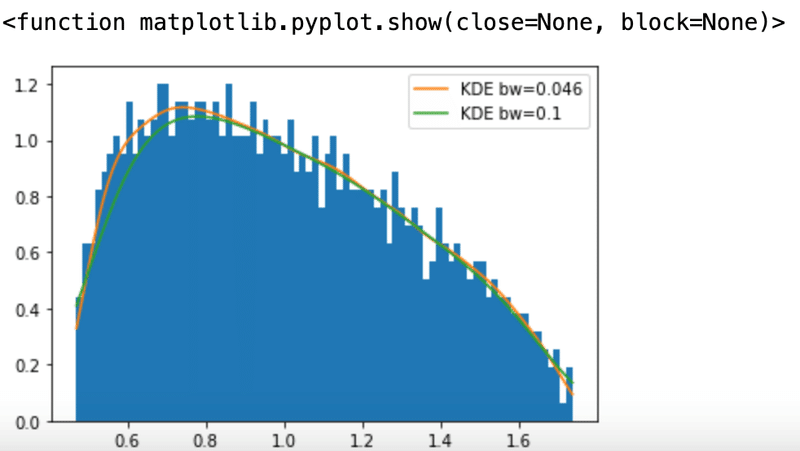
この記事が気に入ったらサポートをしてみませんか?